PIC benchmark of particle-core model

A simple one-dimensional particle-core (PC) model shows that particles can be driven to large amplitudes through a parametric resonance with the core oscillations. Here we benchmark the model against particle-in-cell (PIC) simulations of a KV distribution in a continuous focusing channel. The simulation is built using PyORBIT, an s-based PIC code.

import numpy as np
import matplotlib.pyplot as plt
import scipy.constants
import scipy.signal

# PyORBIT
from orbit.core.bunch import Bunch
from orbit.core.spacecharge import SpaceChargeCalc2p5D
from orbit.space_charge.sc2p5d import setSC2p5DAccNodes
from orbit.teapot import ContinuousLinearFocusingTEAPOT
from orbit.teapot import TEAPOT_Lattice
from orbit.utils.consts import mass_proton

# local
import pcm
from diag import BunchHistCalc
from utils import intensity_from_perveance
from utils import samp_dist

diag.py

"""PyORBIT diagnostics."""
import copy

import numpy as np

from orbit.core.bunch import Bunch
from orbit.core.spacecharge import Grid1D
from orbit.core.spacecharge import Grid2D


def get_grid_points(grid_coords: list[np.ndarray]) -> np.ndarray:
    if len(grid_coords) == 1:
        return grid_coords[0]
    return np.vstack([c.ravel() for c in np.meshgrid(*grid_coords, indexing="ij")]).T


def grid_edges_to_coords(grid_edges: np.ndarray) -> np.ndarray:
    return 0.5 * (grid_edges[:-1] + grid_edges[1:])


def grid_coords_to_edges(grid_coords: np.ndarray) -> np.ndarray:
    delta = grid_coords[1] - grid_coords[0]
    grid_edges = np.zeros(grid_coords.shape[0] + 1)
    grid_edges[0] = grid_coords[0] - 0.5 * delta
    grid_edges[1:] = grid_coords + 0.5 * delta
    return grid_edges


def make_grid(shape: tuple[int, ...], limits: list[tuple[float, float]]) -> Grid2D:
    if len(shape) == 1:
        return Grid1D(shape[0], limits[0][0], limits[0][1])
    elif len(shape) == 2:
        return Grid2D(
            shape[0] + 1,
            shape[1] + 1,
            limits[0][0],
            limits[0][1],
            limits[1][0],
            limits[1][1],
        )
    else:
        raise ValueError


class Histogram:
    def __init__(self, values: np.ndarray, edges: np.ndarray = None, coords: np.ndarray = None) -> None:
        self.values = np.copy(values)

        self.coords = coords
        self.edges = edges
        if self.coords is None and self.edges is not None:
            self.coords = [grid_edges_to_coords(e) for e in self.edges]
        if self.edges is None and self.coords is not None:
            self.edges = [grid_coords_to_edges(c) for c in self.coords]

        self.coords = [np.copy(_) for _ in self.coords]
        self.edges = [np.copy(_) for _ in self.edges]

    def copy(self):
        return copy.deepcopy(self)


class BunchHistCalc:
    def __init__(
        self,
        axis: tuple[int, ...],
        shape: tuple[int, ...],
        limits: list[tuple[float, float]],
    ) -> None:
        self.axis = axis
        self.ndim = len(axis)

        self.dims = ["x", "xp", "y", "yp", "z", "dE"]
        self.dims = [self.dims[i] for i in self.axis]

        self.grid_shape = shape
        self.grid_limits = limits
        self.grid_edges = [
            np.linspace(self.grid_limits[i][0], self.grid_limits[i][1], self.grid_shape[i] + 1)
            for i in range(self.ndim)
        ]
        self.grid_coords = [grid_edges_to_coords(e) for e in self.grid_edges]
        self.grid_values = np.zeros(shape)
        self.grid_points = get_grid_points(self.grid_coords)
        self.grid = make_grid(self.grid_shape, self.grid_limits)

        self.inv_cell_volume = np.prod([e[1] - e[0] for e in self.grid_edges])

    def bin_bunch(self, bunch: Bunch) -> None:
        macrosize = bunch.macroSize()
        if macrosize == 0:
            bunch.macroSize(1.0)
        
        self.grid.binBunch(bunch, *self.axis)

        bunch.macroSize(macrosize)

    def compute_histogram(self, bunch: Bunch) -> np.ndarray:
        self.bin_bunch(bunch)

        values = np.zeros(self.grid_points.shape[0])
        for i, indices in enumerate(np.ndindex(*self.grid_shape)):
            values[i] = self.grid.getValueOnGrid(*indices)
        return values.reshape(self.grid_shape)

    def __call__(self, bunch: Bunch) -> Histogram:
        self.grid.setZero()
        self.grid_values = self.compute_histogram(bunch)
        return Histogram(values=self.grid_values, edges=self.grid_edges)

pcm.py

"""One-dimensional particle-core model in continuous-focusing channel [1].

[1] Wangler, T. P., et al. "Particle-core model for transverse dynamics of beam
    halo." Physical review special topics-accelerators and beams 1.8 (1998):
    084201.
"""

import numpy as np
import scipy.integrate


def get_eq_radius(emittance: float, k: float) -> float:
    return np.sqrt(emittance / k)


def get_eq_perveance(emittance: float, k: float, k0: float) -> float:
    radius = get_eq_radius(emittance, k)
    return (k0**2 - k**2) * radius**2


def get_eq_cov_matrix(radius: float, emittance: float) -> np.ndarray:
    """Return 4x4 covariance matrix for round beam at equilibrium."""
    cov_matrix = np.zeros((4, 4))
    cov_matrix[0, 0] = 0.25 * radius**2
    cov_matrix[2, 2] = cov_matrix[0, 0]
    cov_matrix[1, 1] = (0.25 * emittance) ** 2 / cov_matrix[0, 0]
    cov_matrix[3, 3] = cov_matrix[1, 1]
    return cov_matrix


def get_cov_matrix(radius: float, radius_prime: float, eta: float) -> np.ndarray:
    cov_matrix = np.zeros((2, 2))
    cov_matrix[0, 0] = radius**2
    cov_matrix[0, 1] = cov_matrix[1, 0] = radius * radius_prime
    cov_matrix[1, 1] = (eta / radius)**2 + radius_prime**2
    return cov_matrix * 0.25


def get_ellipse_params(cov_matrix: np.ndarray) -> tuple[float, float, float]:
    sii = cov_matrix[0, 0]
    sjj = cov_matrix[1, 1]
    sij = cov_matrix[0, 1]
    angle = -0.5 * np.arctan2(2 * sij, sii - sjj)
    _sin = np.sin(angle)
    _cos = np.cos(angle)
    _sin2 = _sin**2
    _cos2 = _cos**2
    rx = np.sqrt(abs(sii * _cos2 + sjj * _sin2 - 2 * sij * _sin * _cos))
    ry = np.sqrt(abs(sii * _sin2 + sjj * _cos2 + 2 * sij * _sin * _cos))
    return (rx, ry, angle)


def ode_system(t: float, v: np.ndarray, eta: float) -> np.ndarray:
    """ODE system for 1D particle-core model in linear continuous-focusing lattice.

    Args:
        t: Dimensionless time coordinate.
            t = s * k0, where s is distance and k0 is lattice wavenumber.
        v: Vector of envelope and particle states.
            v[0] = Envelope radius R (scaled by equilibrium radius R0).
            v[1] = dR/dt.
            v[2] = particle x (scaled by R0).
            v[3] = dx/dt.
            ...
        eta: Tune depression ratio k / k0.

    Returns:
        dv/dt
    """
    r, rp, x, xp = v

    f_sc = 0.0
    if abs(x) <= r:
        f_sc = x / r**2
    else:
        f_sc = 1.0 / x

    vp = np.zeros_like(v)
    vp[0] = rp
    vp[1] = -r + (eta**2 / r**3) + ((1.0 - eta**2) / r)
    vp[2] = xp
    vp[3] = -x + (1.0 - eta**2) * f_sc
    return vp


def track(
    envelope: np.ndarray,
    particles: np.ndarray,
    eta: float,
    t_max: float,
    t_steps: float,
) -> dict[str, np.ndarray]:
    """Track particle-core system.

    Args:
        envelope: Initial envelope r and dr/dt.
        particles: Initial particle x and dx/dt coordinates, shape (n, 2).
        eta: Tune depression ratio.
        t_max: Evolution time.
        t_steps: Number of evaluation points along t axis.
    Returns:
        history: Dictionary with the following keys:
            - "t": time
            - "r": envelope r, shape (t_steps + 1).
            - "rp": envelope dr/dt, shape (t_steps + 1).
            - "particles": particle coordinates, shape (t_steps + 1, n, 2).
    """
    solutions = []
    for particle in particles:
        solution = scipy.integrate.solve_ivp(
            ode_system,
            t_span=(0.0, t_max),
            t_eval=np.linspace(0.0, t_max, t_steps + 1),
            y0=np.hstack([envelope, particle]),
            args=(eta,),
            method="LSODA",
            rtol=1e-8,
            atol=1e-8,
        )
        solutions.append(solution)

    history = {}
    history["t"] = solution.t
    history["r"] = solution.y[0]
    history["rp"] = solution.y[1]
    history["particles"] = np.zeros((t_steps + 1, particles.shape[0], particles.shape[1]))
    for index, solution in enumerate(solutions):
        history["particles"][:, index, :] = np.transpose(solution.y[2:])
    return history


def track_strobe(
    envelope: np.ndarray,
    particles: np.ndarray,
    eta: float,
    periods: int,
    phase: str = "min",
) -> dict[str, np.ndarray]:
    """Track particle-core system - evaluate at minima of core radius.

    Args:
        envelope: Initial envelope r and dr/dt.
        particles: Initial particle x and dx/dt coordinates, shape (n, 2).
        eta: Tune depression ratio.
        periods: Number of envelope oscillation periods (approximate).
        phase: Whether to evaluate system at minimum or maximum beam size {"min", "max"}.
            Uses `events` parameter of `scipy.integrate.solve_ivp` to determine
            evaluation points rather than setting integration period. (Accounts for
            slight differences from theoretical envelope oscillation period.)
    Returns:
        history: Dictionary with the following keys:
            - "t": time
            - "r": envelope r, shape (t_steps + 1).
            - "rp": envelope dr/dt, shape (t_steps + 1).
            - "particles": particle coordinates, shape (t_steps + 1, n, 2).
    """

    def event_func(t: float, y: np.ndarray, eta: float) -> float:
        return y[1] if phase == "min" else -y[1]

    event_func.direction = 1

    wavenumber = np.sqrt(2.0 * (1.0 + eta**2))  # breathing mode (approximate)
    wavelength = 2.0 * np.pi / wavenumber
    t_max = periods * wavelength

    envelope = np.copy(envelope)
    if envelope[0] == 1.0:
        envelope[0] += 0.01

    solutions = []
    for particle in particles:
        solution = scipy.integrate.solve_ivp(
            ode_system,
            t_span=(0.0, t_max),
            y0=np.hstack([envelope, particle]),
            args=(eta,),
            events=event_func,
            method="LSODA",
            rtol=1e-8,
            atol=1e-8,
        )
        solutions.append(solution)

    history = {}
    history["t"] = solution.t_events[0]
    history["r"] = solution.y_events[0][:, 0]
    history["rp"] = solution.y_events[0][:, 1]
    history["particles"] = np.zeros((solution.y_events[0].shape[0], particles.shape[0], particles.shape[1]))
    for index, solution in enumerate(solutions):
        history["particles"][:, index, :] = solution.y_events[0][:, 2:]
    return history

utils.py

"""Utility functions."""
def samp_dist(
    size: int,
    name: str = "kv",
    cov_matrix: np.ndarray = None,
    seed: int = None,
    dim: int = 4,
):
    """Sample particles from ellipsoidally symmetric distribution function.

    Parameters:
        name: Distribution name {"kv", "waterbag", "gauss"}.
        cov_matrix: Covariance matrix, shape (dim, dim).
        seed: Random number generator seed.
        dim: Number of dimensions.

    Returns:
        Particle coordinates, shape (size, dim).
    """
    rng = np.random.default_rng(seed)

    if name == "gauss":
        x = rng.normal(size=(size, dim))
    elif name == "kv":
        x = rng.normal(size=(size, dim))
        x = x / np.linalg.norm(x, axis=1, keepdims=True)
        x = x / np.std(x, axis=0)
    elif name == "waterbag":
        x = rng.normal(size=(size, 4))
        x = x / np.linalg.norm(x, axis=1, keepdims=True)
        r = rng.uniform(0.0, 1.0, size=size) ** (1.0 / dim)
        x = x * r[:, None]
        x = x / np.std(x, axis=0)
    else:
        raise ValueError

    if cov_matrix is not None:
        x = x @ np.linalg.cholesky(cov_matrix)
    return x


def get_classical_radius() -> float:
    """Return classical proton radius [m]."""
    m = scipy.constants.proton_mass
    q = scipy.constants.elementary_charge
    c = scipy.constants.speed_of_light
    eps0 = scipy.constants.epsilon_0
    return q**2 / (4.0 * np.pi * eps0 * m * c**2)


def intensity_from_perveance(
    perveance: float, kin_energy: float, rest_energy: float, length: float
) -> float:
    """Return beam intensity from perveance, energy, mass, and length.""" 
    gamma = 1.0 + (kin_energy / rest_energy)
    beta = math.sqrt(1.0 - (1.0 / gamma) ** 2)
    classical_radius = get_classical_radius()
    return length * perveance * beta**2 * gamma**3 / (2.0 * classical_radius)

Set the simulation parameters:

sigma0 = np.radians(80.0)  # phase advance [deg]
eta = 0.5  # tune depression ratio (k / k0)
radius_frac = 0.6095  # initial beam radius / matched radius
emittance = 1e-6  # rms emittance (times 4) [m rad]
bunch_length = 10.0  # bunch length [m]
kin_energy = 0.0025  # kinetic energy [GeV]

# Calculate depressed phase advance
sigma = sigma0 * eta
k0 = sigma0  # wavenumber (assume length = 1 [m])
k = k0 * eta  # depressed wavenumber

# Stationary KV equilibrium parameters
eq_radius = pcm.get_eq_radius(emittance, k)
perveance = pcm.get_eq_perveance(emittance, k, k0)

# Mismatched core radius
radius = eq_radius * radius_frac

# Construct 4 x 4 covariance matrix
cov_matrix = np.zeros((6, 6))
cov_matrix[0:4, 0:4] = pcm.get_eq_cov_matrix(radius, emittance)
cov_matrix[4, 4] = (bunch_length**2) / 12.0  # for uniform density
cov_matrix_init = cov_matrix.copy()

# Get beam intensity from perveance, kinetic energy, mass, and length.
intensity = intensity_from_perveance(perveance, kin_energy, mass_proton, bunch_length)

Find core oscillation wavelength from envelope tracking (ODE solver). For large mismatch this will deviate slightly from the breathing-mode frequency \(k_+^2 = 2 k_0^2 + 2 k^2\). Note that pcm.py uses dimensionless coordinates.

# From small-amplitude perturbation
env_wave_pred = (2.0 * np.pi) / np.sqrt(2.0 * (1.0 + eta**2))

# Track envelope for ~20 core oscillations.
periods = 20
history = pcm.track(
    envelope=np.array([radius_frac, 0.0]),
    particles=np.array([[2.8, 0.0]]),
    eta=eta,
    t_max=(periods * env_wave_pred),
    t_steps=(periods * 100),
)

# Find the peaks
idx, _ = scipy.signal.find_peaks(history["r"])
env_wave_avg = np.mean(np.diff(history["t"][idx]))
env_wave_std = np.std(np.diff(history["t"][idx]))
print("wavelength * k0 (pred) = {:0.4f}".format(env_wave_pred))
print("wavelength * k0 (calc) = {:0.4f} +- {:0.4f}".format(env_wave_avg, env_wave_std))

# Correct wavelength
env_wave = env_wave_avg / k0

wavelength * k0 (pred) = 3.9738
wavelength * k0 (calc) = 3.8566 +- 0.0087

Place a test particle just outside the separatrix and track it for many core oscillations. This forms an approximate upper bound on the halo which can be compared to PIC simulations.

history_pcm = pcm.track_strobe(
    envelope=np.array([radius_frac, 0.0]),
    particles=np.array([[2.8, 0.0]]),  # ~separatrix
    eta=eta,
    periods=500,
)

Set up the PyORBIT simulation.

# Sample particles from 4D KV distribution.
particles = np.zeros((100_000, 6))
particles[:, :4] = samp_dist(
    size=particles.shape[0], name="kv", cov_matrix=cov_matrix_init[:4, :4], seed=14
)
particles[:, 4] = bunch_length * np.random.uniform(-0.5, 0.5, size=particles.shape[0])

# Create bunch object.
bunch = Bunch()
bunch.mass(mass_proton)
bunch.getSyncParticle().kinEnergy(kin_energy)
bunch.macroSize(intensity / particles.shape[0])
for i in range(particles.shape[0]):
    bunch.addParticle(*particles[i])

# Create an accelerator lattice with a continuous-focusing node.
lattice = TEAPOT_Lattice()
lattice.addNode(ContinuousLinearFocusingTEAPOT(length=env_wave, kq=k0**2, nparts=30))

# Add space charge nodes to the lattice.
sc_calc = SpaceChargeCalc2p5D(128, 128, 1)
sc_path_length_min = 0.001
sc_nodes = setSC2p5DAccNodes(lattice, sc_path_length_min, sc_calc)

Track the bunch for 25 periods and record the \(x\)-\(x'\) histogram after each period.

# Set histogram grid limits.
scale = np.array([eq_radius, eq_radius * k0])
xmax = 3.5 * scale
limits = list(zip(-xmax, xmax))

# Create histogram calculator. This grids the particles using PyORBIT `Grid` object.
hist_calc = BunchHistCalc(axis=(0, 1), shape=(150, 150), limits=limits)

# Track the bunch.
histograms = []
for period in range(25 + 1):
    if period > 0:
        lattice.trackBunch(bunch)

    histograms.append(hist_calc(bunch))

I’ll plot the \(x\)-\(x'\) projections in log scale down to \(10^{-3}\) as a fraction of the peak density. The PC model result for a particle just outside the separatrix is shown in red.

import os

os.makedirs("outputs", exist_ok=True)

for i, histogram in enumerate(histograms):
    values = histogram.values.copy()
    values = values / np.max(values)
    values = np.ma.log10(values)

    fig, ax = plt.subplots(figsize=(5, 4))
    ax.set_xlabel("$x / r_0$")
    ax.set_ylabel(r"$x' / k_0 r_0$")
    ax.set_title(f"Period = {i}", fontsize="medium")
    ax.scatter(
        history_pcm["particles"][..., 0],
        history_pcm["particles"][..., 1],
        ec="none",
        s=1,
        c="red",
        zorder=9999,
    )
    mesh = ax.pcolormesh(
        histogram.edges[0] / scale[0],
        histogram.edges[1] / scale[1],
        values.T,
        cmap="Greys",
        vmin=-3.0,
    )
    fig.colorbar(mesh)

    plt.savefig(f"outputs/hist_{i:02.0f}.png", dpi=125)
    plt.close()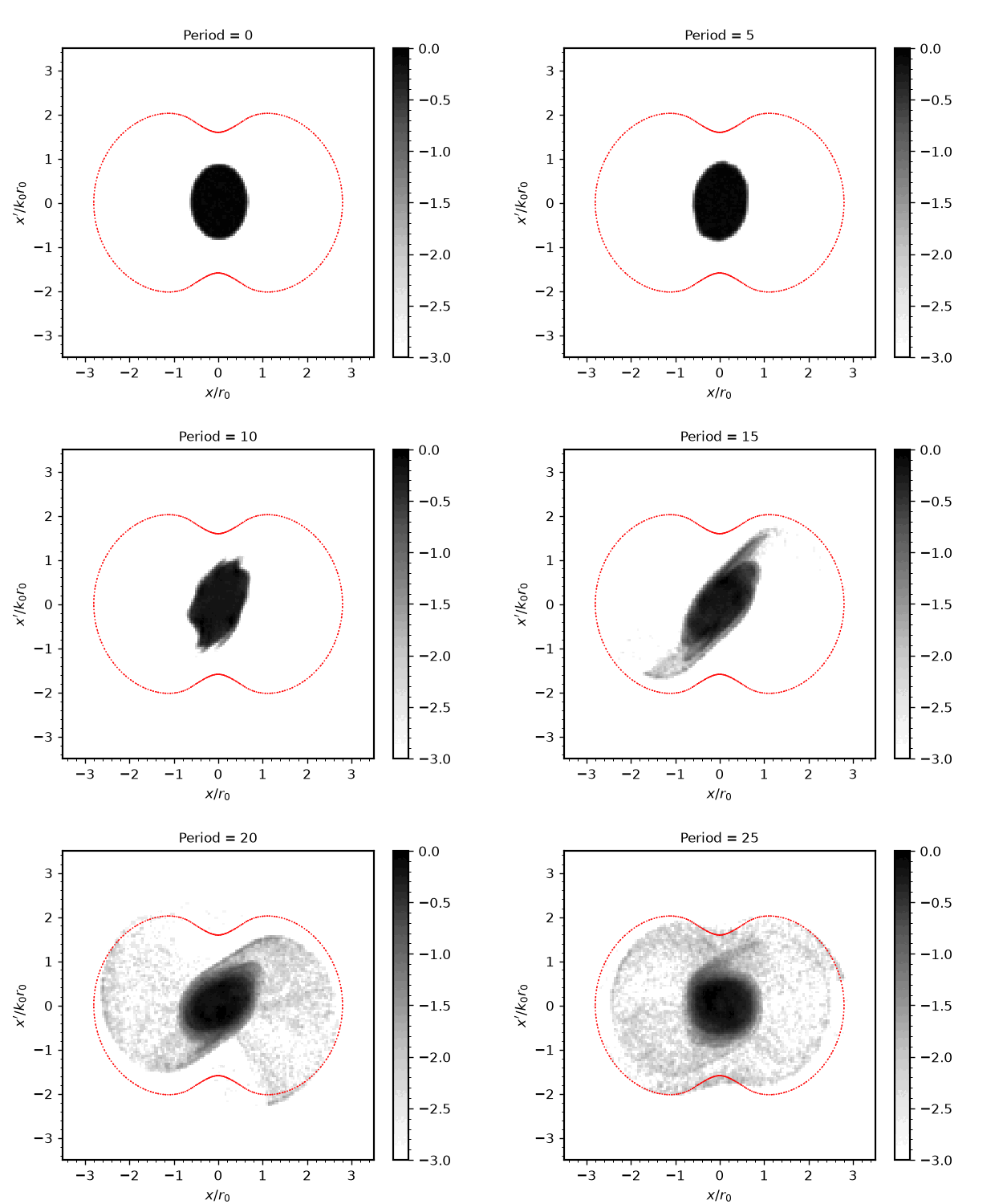

In this case the KV distribution is unstable, which can only be described with a full kinetic model. But the 2:1 parametric resonance is still the dominant machanism of halo formation after the beam deviates from equilibrium, and the halo boundary is well-described by the particle-core model.

Note that the distribution rotates by \(\approx\) 180 degrees on each frame of the animation. This is because each frame occurs at the minimum of the core oscillations, and many of the particles oscillate at around half the core oscillation frequency when they are driven to the halo.