Eigenpainting: a method to mitigate space charge in high-intensity hadron beams
Our paper, Demonstration of a novel phase-space painting method in a coupled lattice to mitigate space charge in high-intensity hadron beams, was recently accepted by Physical Review Letters (PRL). Here’s the preprint. The paper presents the first experimental test of eigenpainting, a method proposed by Viatcheslav (Slava) Danilov in 2003 [1].1 In this post, I’ll share some additional background and figures to help explain our results.
Introduction
Accelerators such as the SNS and J-PARC use charge-exchange injection to create intense proton beams for neutron scattering experiments. The injection is a three-step process: H- (negative hydrogen) ions are accelerated in a linac, converted to protons using a carbon foil or laser-magnet system, and then transferred to an accumulator ring. We call each batch of injected protons a minipulse. After the first minipulse completes one lap around the ring, a second is injected, and so on for hundreds or thousands of turns.
Vanilla charge-exchange injection leads to charge pile-up at the injection point, causing halo formation and beam loss. This motivates the technique of phase space painting: moving the injection point in phase space (position-momentum space) during accumulation. Painting spreads the charge over a larger area, reducing peak density and associated space charge effects. Painting can also enable more detailed control of the distribution, although this is challenging because each injected minipulse affects the beam dynamics on the next turn.
Eigenpainting is a method to paint stationary phase space distributions. The method follows from the eigenvector analysis of coupled motion, which I’ll summarize in Section 2. In Section 3, I’ll describe several possible applications of eigenpainting. Finally, in Section 4, I’ll describe our attempt to implement eigenpainting in the SNS and our plans for follow-up experiments.
Eigenvectors, eigenvalues, and eigenpainting
Eigenvector analysis
Assume the phase space coordinates \(\mathbf{x}\) evolve according to
\[ \mathbf{x} \rightarrow \mathbf{M} \mathbf{x} , \tag{1}\]
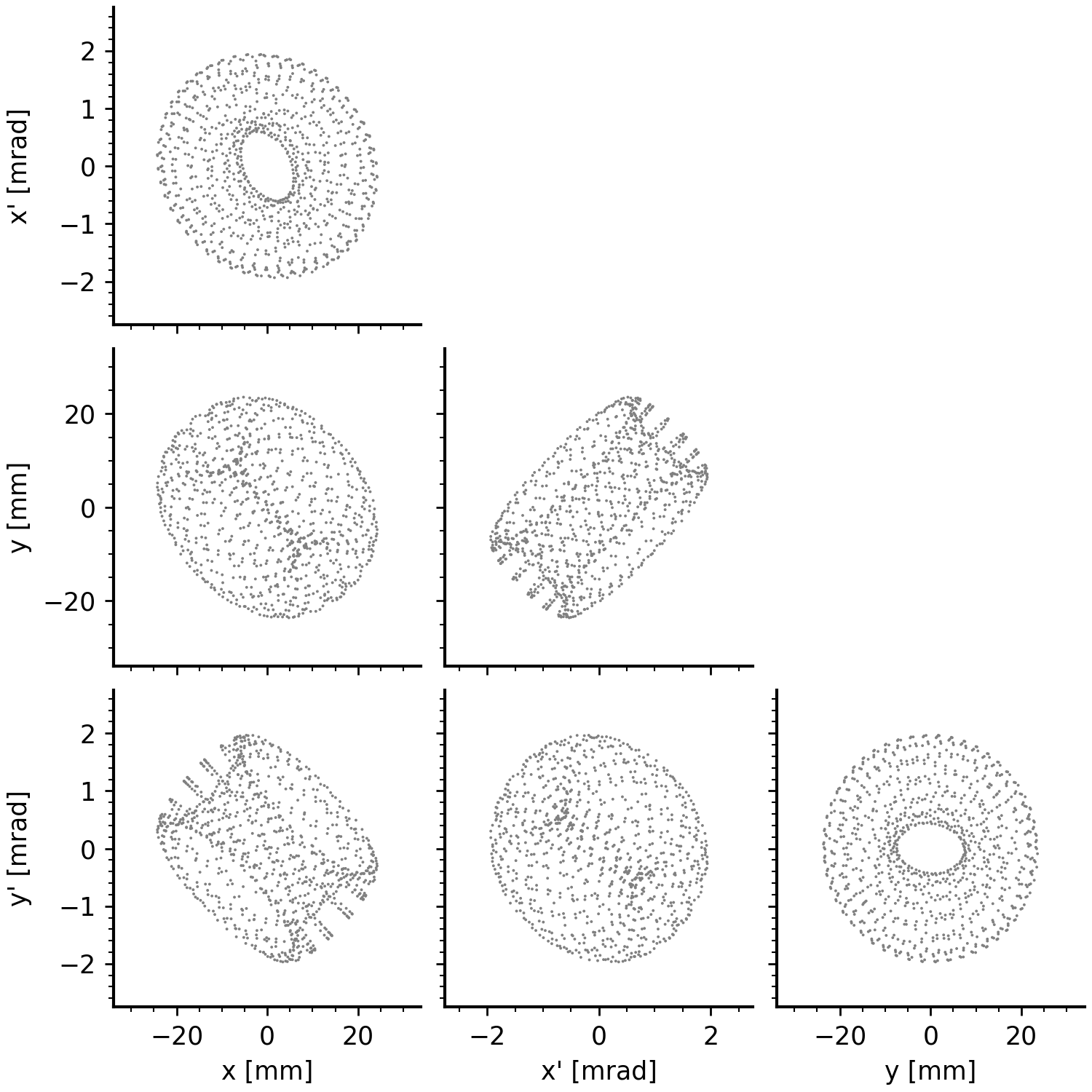
where \(\mathbf{M}\) is a symplectic matrix and \(\rightarrow\) represents tracking through one turn in the ring. For example, Figure 1 shows a particle’s coordinates over 1000 turns in the SNS ring.
We can simplify the motion using the eigenvectors of the transfer matrix. The eigenvectors solve
\[ \mathbf{Mv}_k = e^{-i\mu_k} \mathbf{v}_k , \tag{2}\]
where \(k = 1, 2\). Since the eigenvectors form a basis, we can write the phase space coordinate vector as
\[ \mathbf{x} = \text{Re} \left\{ \sqrt{2 J_1} \mathbf{v}_1 e^{-i\psi_1} + \sqrt{2 J_2} \mathbf{v}_2 e^{-i\psi_2} \right\} . \tag{3}\]
Here, \(J_{1, 2}\) are initial amplitudes, \(\psi_{1, 2}\) are initial phases, and \(\text{Re}\{\dots\}\) selects the non-imaginary component. The transfer matrix simply adds a phase to each eigenvector:
\[ \mathbf{Mx} = \text{Re} \left\{ \sqrt{2 J_1}\mathbf{v}_1 e^{-i\left(\psi_1 + \mu_1\right)} + \sqrt{2 J_2}\mathbf{v}_2 e^{-i(\psi_2 + \mu_2)} \right\}. \tag{4}\]
The amplitudes \(J_{1, 2}\) are therefore invariants of the motion.
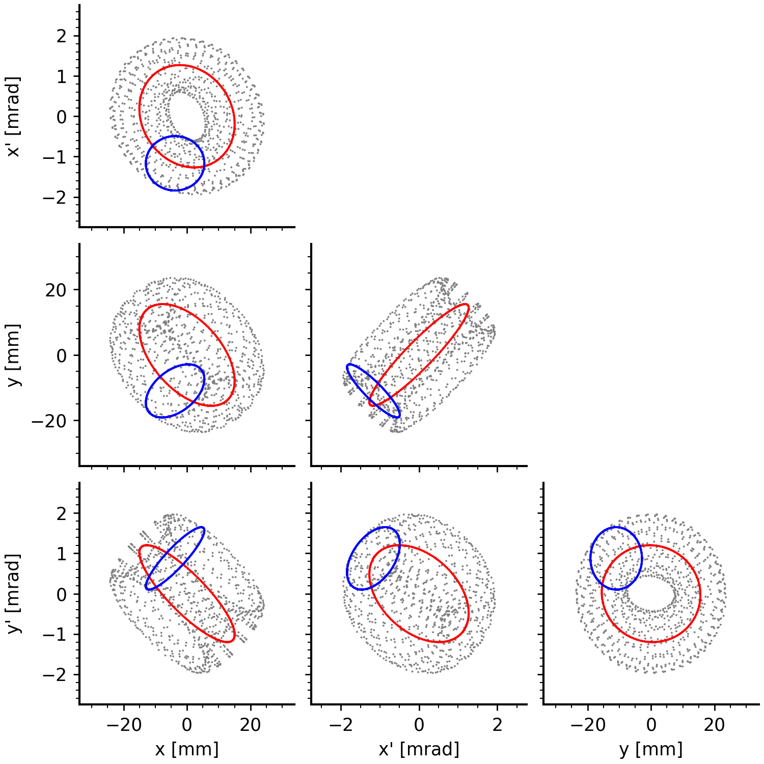
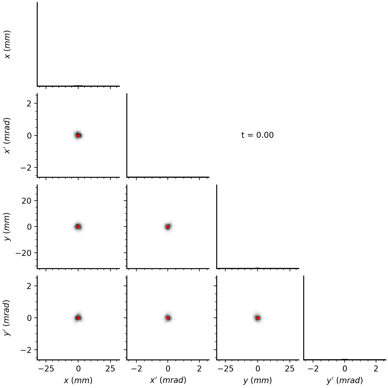
At a fixed point in the ring, the real component of \(\mathbf{v}_k\) traces a two-dimensional ellipse of area \(2 J_k\) at frequency \(\mu_k / 2\pi\). This is shown in Figure 2. If there is no coupling in the lattice, the first ellipse will align with the \(x\)-\(x'\) axis and the second with the \(y\)-\(y'\) axis; otherwise, the ellipses can have different orientations in the four-dimensional phase space.
Normalized coordinates
We can use the eigenvectors to construct a symplectic matrix \(\mathbf{V}\),
\[ \mathbf{V} = \left[ +\Re\{\mathbf{v}_1\} -\Im\{\mathbf{v}_1\} +\Re\{\mathbf{v}_2\} -\Im\{\mathbf{v}_2\} \right] , \tag{5}\]
that converts \(\mathbf{M}\) to block-diagonal form:
\[\mathbf{V^{-1} M V} = \begin{bmatrix} \cos{\mu_1} & \sin{\mu_1} & 0 & 0 \\ -\sin{\mu_1} & \cos{\mu_1} & 0 & 0 \\ 0 & 0 & \cos{\mu_2} & \sin{\mu_2} \\ 0 & 0 & -\sin{\mu_2} & \cos{\mu_2} \end{bmatrix} . \tag{6}\]
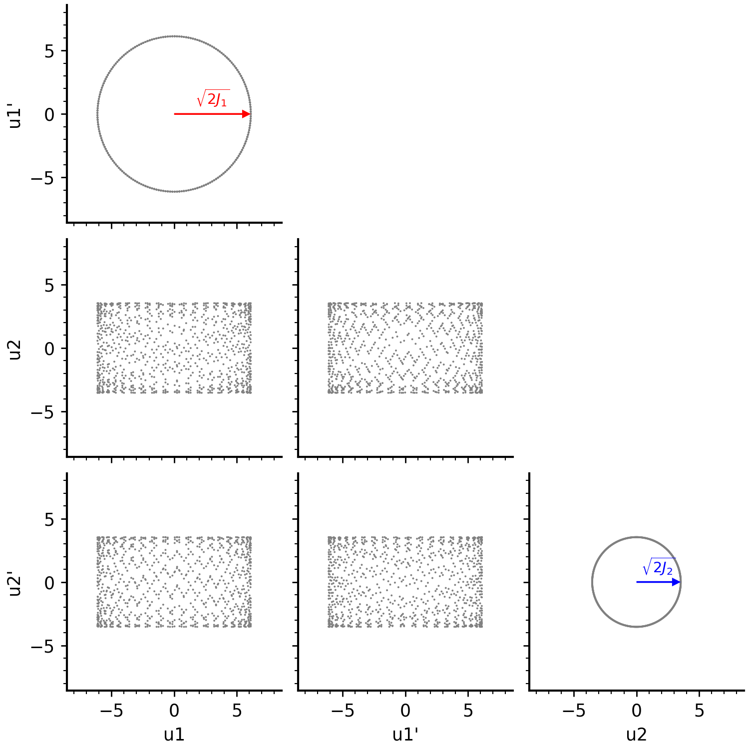
In the “normalized” coordinates \(\mathbf{u} = \mathbf{V}^{-1} \mathbf{x}\), the particle simply rotates in each phase plane, tracing circles of area \(2 J_k\) at frequencies \(\mu_k\). The cross-plane projections are rectangular because there is no coupling in the normalized frame.
\[ \mathbf{u} = \begin{bmatrix} +\sqrt{2J_1}\cos{(\psi_1 + \mu_1)} \\ -\sqrt{2J_1}\sin{(\psi_1 + \mu_1)} \\ +\sqrt{2J_2}\cos{(\psi_2 + \mu_2)} \\ -\sqrt{2J_2}\sin{(\psi_2 + \mu_2)} \end{bmatrix}. \tag{7}\]
Single-mode injection painting
The idea behind eigenpainting is to inject particles into only one mode, i.e., along only one eigenvector. Suppose we continuously inject particles at a fixed amplitude \(J_1\) and phase \(\psi_1\). The injected particles will advance in phase, eventually filling the ellipse traced by the eigenvector. If we inject particles at a different amplitude, they will form another ellipse. Thus, by varying the injection amplitude as a function of time, we can build any elliptically symmetric distribution \(f(J_1)\).
We’ll focus on the specific choice of linearly increasing amplitude:
\[ \begin{aligned} J_1(t) &= \tilde{J}_1 t , \\ J_2(t) &= 0 , \end{aligned} \tag{8}\]
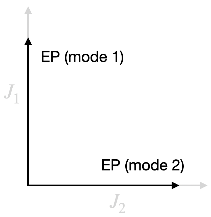
where \(t\) is the time, scaled to the range [0, 1], and \(\tilde{J}_1\) is a maximum value of \(J_1\). We could also paint into the other mode by swapping \(J_1\) and \(J_2\). We can represent the painting path as a curve in the \(J_1\)-\(J_2\) space:
In normalized coordinates, the distribution will look like this:
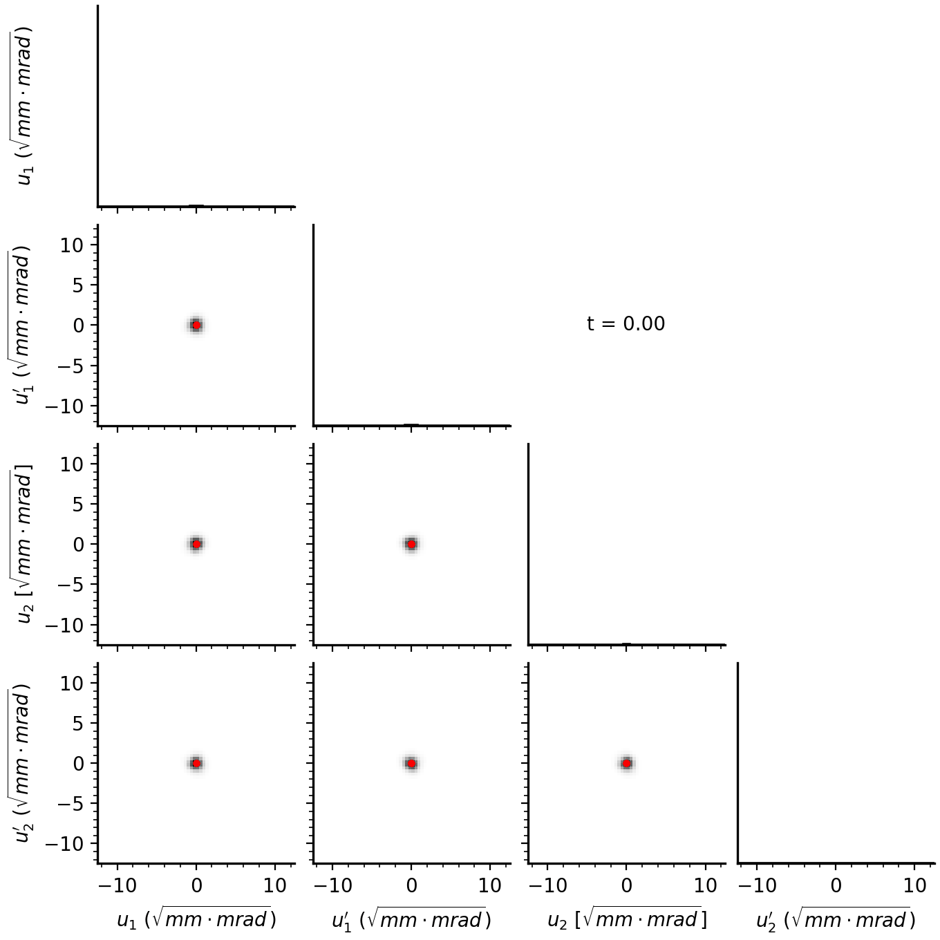
The linear amplitude scaling forms a uniform disk in the first phase plane, while particles in the second phase plane are concentrated at the origin. In reality, the injected minipulse has a finite size, so we end up with a small blob.
The actual distribution will depend on \(\mathbf{V}\), which encodes the structure of the accelerator lattice. For example, Figure 5 shows the result of painting into the SNS ring.
Space charge typically invalidates methods based on single-particle, linear dynamics. Incredibly, eigenpainting still works. The painted distribution projects to a uniform density within an elliptical envelope, generating an electric field with linear space charge forces. Space charge simply modifies the transfer matrix \(\mathbf{M}\) to a new effective transfer matrix \(\hat{\mathbf{M}}\). We can construct a normalization matrix \(\hat{\mathbf{V}}\) from \(\hat{\mathbf{M}}\) and run eigenpainting as before.
Another critical point is that the painted distribution is stationary with respect to turn number. The painted distribution is an equilibrium solution of the Vlasov-Poisson equations, known as the KV distribution [4]. Equilibrium distributions are functions of invariants (\(J_1\) in this case) and preserve their functional form in phase space as they evolve. This ensures the linearity of space charge forces throughout the ring. Furthermore, the distribution is in equilibrium at all times \(t\); the only change is a global scaling factor as particles are added to the edge of the beam ellipse.
Applications of eigenpainting
Now that eigenpainting is defined, let’s discuss what it could be used for. We’ll focus on three features of the accumulated distribution: small four-dimensional emittance, strong cross-plane correlations, and uniform density.
Emittance as a measure of phase space volume
Emittance is a measure of phase space volume calculated from the covariance matrix \(\mathbf{\Sigma}\):
\[ \mathbf{\Sigma} = \langle \mathbf{x} \mathbf{x}^T \rangle \begin{bmatrix} \langle{xx}\rangle & \langle{xx'}\rangle & \langle{xy}\rangle & \langle{xy'}\rangle \\ \langle{x'x}\rangle & \langle{x'x'}\rangle & \langle{x'y}\rangle & \langle{x'y'}\rangle \\ \langle{yx}\rangle & \langle{yx'}\rangle & \langle{yy}\rangle & \langle{yy'}\rangle \\ \langle{y'x}\rangle & \langle{y'x'}\rangle & \langle{y'y}\rangle & \langle{y'y'}\rangle \end{bmatrix} , \tag{9}\]
where \(x\)-\(y\) are the transverse positions, \(x'\)-\(y'\) are the velocities, and \(\langle \dots \rangle\) is an average over all particles. The covariance matrix defines an ellipsoid from the expression \(\mathbf{x}^T \mathbf{\Sigma}^{-1} \mathbf{x} = 1\). The four-dimensional emittance \(\varepsilon_{4D}\) is the volume of this ellipsoid:
\[ \varepsilon_{4D} = \sqrt{\det{\mathbf{\Sigma}}}. \tag{10}\]
From Liouville’s Theorem, the four-dimensional emittance is conserved under linear symplectic transformations. We can also write the four-dimensional emittance as the product of the intrinsic emittances \(\varepsilon_{1, 2}\), which are individually conserved:
\[ \varepsilon_{4D} = \varepsilon_{1}\varepsilon_{2} . \]
The intrinsic emittances are calculated from a symplectic diagonalization of \(\mathbf{\Sigma}\):
\[ \mathbf{\Sigma} = \mathbf{V} \begin{bmatrix} \varepsilon_1 & 0 & 0 & 0 \\ 0 & \varepsilon_1 & 0 & 0 \\ 0 & 0 & \varepsilon_2 & 0 \\ 0 & 0 & 0 & \varepsilon_2 \end{bmatrix} \mathbf{V}^T , \tag{11}\]
where \(\mathbf{V}\) is a symplectic matrix. It’s no coincidence that \(\mathbf{V}\) was also the symbol used for the normalization matrix calculated from the lattice eigenvectors. There’s a close connection between the two. Both matrices define a “normalized” coordinate system. The \(\mathbf{V}\) in Equation 11 is also constructed from a set of eigenvectors, but this time the eigenvectors solve
\[ \mathbf{\Sigma}\mathbf{U} \mathbf{v}_k = i \varepsilon_k \mathbf{v}_k , \tag{12}\]
where \(\mathbf{U}\) is the Poisson matrix: \[ \mathbf{U} = \begin{bmatrix} 0 & +1 & 0 & 0 \\ -1 & 0 & 0 & 0 \\ 0 & 0 & 0 & +1 \\ 0 & 0 & -1 & 0 \\ \end{bmatrix} . \tag{13}\]
These “beam eigenvectors” define a symplectic transformation that removes all linear cross-plane correlations in the beam while preserving the intrinsic emittances; for example, mapping Figure 5 to Figure 4. Compare to the “lattice eigenvectors”, which define a transformation that removes all cross-plane correlations in the external focusing fields. If the “beam eigenvectors” are the same as the “lattice eigenvectors”, then the two \(\mathbf{V}\) matrices are identical, and the covariance matrix is invariant with respect to turn number:
\[ \mathbf{\Sigma} \rightarrow \mathbf{M} \mathbf{\Sigma} \mathbf{M}^T = \mathbf{\Sigma} . \tag{14}\]
Such a beam is matched to the lattice.2 In this case, the intrinsic emittances \(\varepsilon_k\) calculate the spread of amplitudes \(J_k\), or the rms area of the projected ellipse in the \(u_k\)-\(u_k'\) plane (Figure 4). For this reason, the intrinsic emittances are also called the eigenemittances or mode emittances.
In addition to the intrinsic emittances, we can define the projected emittances \(\varepsilon_{x, y}\):
\[ \begin{aligned} \varepsilon_x &= \sqrt{\det{\mathbf{\Sigma}_{xx}}} , \\ \varepsilon_y &= \sqrt{\det{\mathbf{\Sigma}_{yy}}} , \\ \end{aligned} \tag{15}\]
where
\[ \mathbf{\Sigma} = \begin{bmatrix} \mathbf{\Sigma}_{xx} & \mathbf{\Sigma}_{xy} \\ \mathbf{\Sigma}_{xy}^T & \mathbf{\Sigma}_{yy} \end{bmatrix} . \tag{16}\]
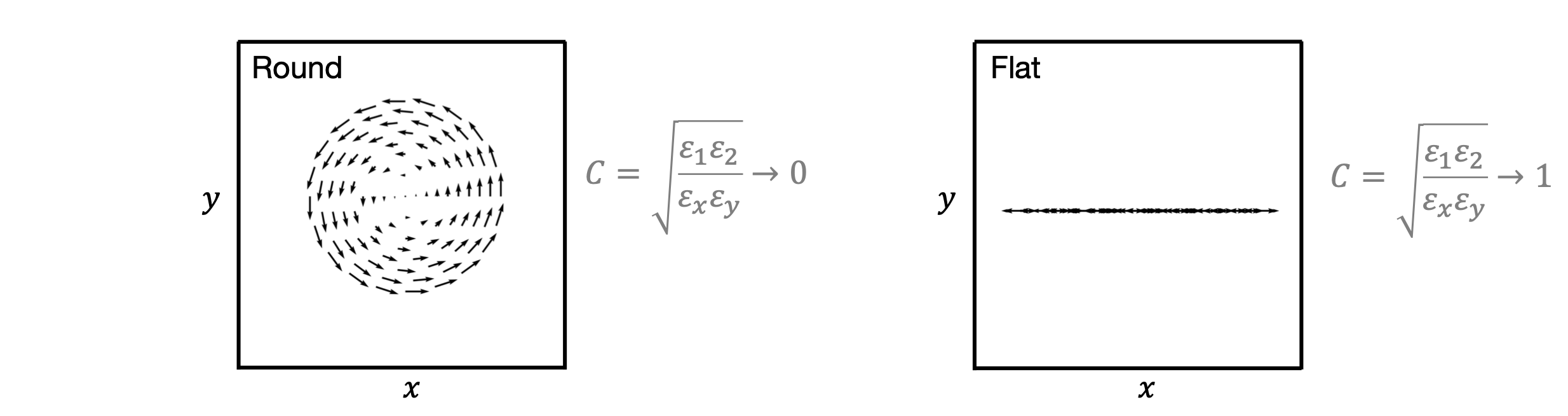
The projected emittances define the rms ellipse areas in the \(x\)-\(x'\) and \(y\)-\(y'\) planes. Thus, the projected emittance ratio \(\varepsilon_x / \varepsilon_y\) tells us the fraction of particles that occupy the horizontal mode compared to the vertical mode of oscillation. The intrinsic emittances have a similar interpretation. The intrinsic emittance ratio \(\varepsilon_1 / \varepsilon_2\) tells us the fraction of particles that occupy one mode compared to another mode of oscillation, where the modes are defined by the symplectic matrix \(\mathbf{V}\) in Equation 11. For example, if \(\mathbf{V}\) is the identity matrix, then the two modes correspond to \(x\) and \(y\). In general, the modes correspond to elliptical trajectories in the \(x\)-\(y\) plane.
Flat beams for high-energy colliders
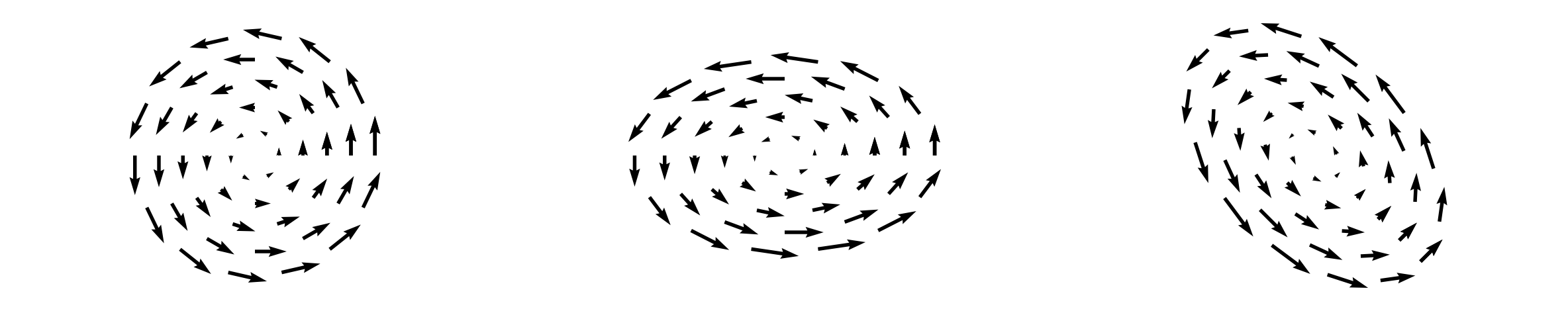
The eigenpainted beam has a very large ratio of intrinsic emittances: \(\varepsilon_1 \gg \varepsilon_2\); therefore, the particle motion is dominated by a single elliptical mode. I’ll call this a vortex distribution referring to the spiral pattern of the velocity field.3 Note that a vortex distribution can have any distribution in the \(x\)-\(y\) plane; the important part is the velocity.
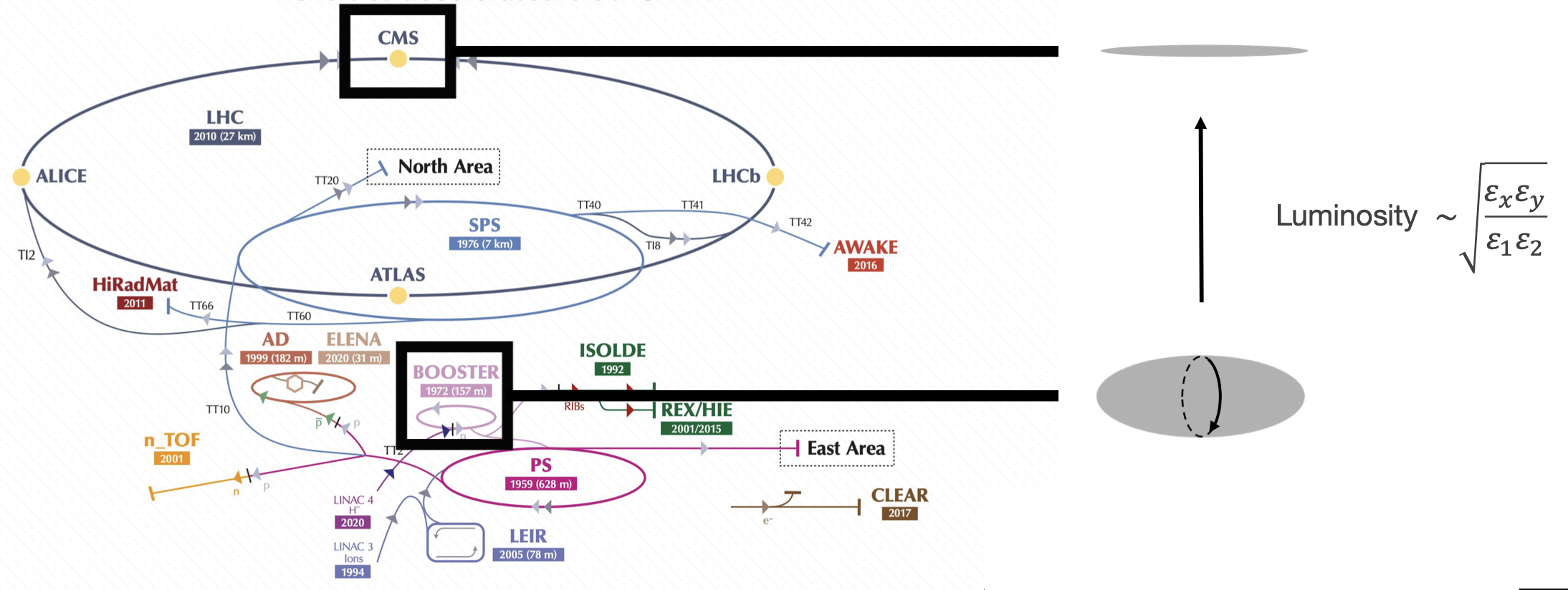
Vortex distributions could be used to increase luminosity in high-energy colliders [5]. To maximize the luminosity (the number of collisions per unit time per unit area), we want to maximize the particle density at the collision point. Unfortunately, the density is fundamentally limited by space charge forces during the low-energy stages of acceleration. But we can play a trick: we can accumulate a round vortex beam, accelerate it to high energy, and then remove its angular momentum using a series of skew quadrupoles. The skew quadrupoles simply map the projected emittances \(\varepsilon_{x, y}\) to the intrinsic emittances \(\varepsilon_{1, 2}\). If the initial beam has a large intrinsic emittance ratio, the final beam will have a large projected emittance ratio. This is the so-called round-to-flat (RTF) transformation [6] shown in Figure 7. Since inter-particle forces are negligible at higher energies, this scheme essentially bypasses the space charge limit on the beam density.
Vortex distributions for space charge mitigation
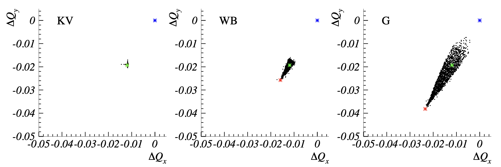
Vortex distributions could also mitigate space charge effects. Consider a simplified model that represents the beam as a frozen background potential \(\phi(x, y)\). In a Gaussian distribution, the potential contains terms proportional to \(x^2\), \(x^4\), and so on. These terms act as periodic nonlinear driving forces, leading to resonance at certain frequencies. These resonances are sometimes called space charge structure resonances. The classic example is the fourth-order resonance, which creates four islands in \(x\)-\(x'\) phase space. Recently, Cheon et al. [7] showed that angular momentum can suppress the fourth-order resonance in linear accelerators (Figure 9), and I expect the same could hold in circular accelerators. A pure vortex beam with \(\varepsilon_2 = 0\) is an extreme case of zero relative motion of particles in the beam.
Vlasov-Poisson equilibrium and tune spread minimization
The two eigenpainting applications above do not depend on the spatial density of the bunch; they only require a large intrinsic emittance ratio. A third application that depends on the bunch density is the reduction of tune spread. Space charge shifts the particle tunes (frequencies) based on their location in the bunch. For example, Figure 10 shows the tune spread within a Gaussian distribution. As the intensity increases, the tune spread grows. The danger is that the tunes cross nonlinear resonances driven by nonlinearities in the accelerator lattice. So, at least in this simple model, a smaller tune spread is better.4
The smallest possible tune spread is obtained in a uniform density bunch in which all particles oscillate at the same frequency (left side of Figure 10). The KV distribution is the only arrangement of particles that gives the desired density. It turns out to be impossible to paint a KV distribution with finite emittance in both planes. However, we can paint a KV distribution with zero emittance in one of the planes [4]. This is just what eigenpainting gives us in Figure 5. Note that the zero-emittance plane is not \(x\) or \(y\).
Experimental test of eigenpainting at the SNS
With the background out of the way, I’ll move on to our experiment at the SNS.
In [9], Jeff Holmes ran simulations of the proposed method in the SNS ring.5 He found that even with nonlinearities included, eigenpainting generated a fairly uniform charge density and strong cross-plane correlations. This motivated our experimental program to implement eigenpainting in real life (“in the control room”).
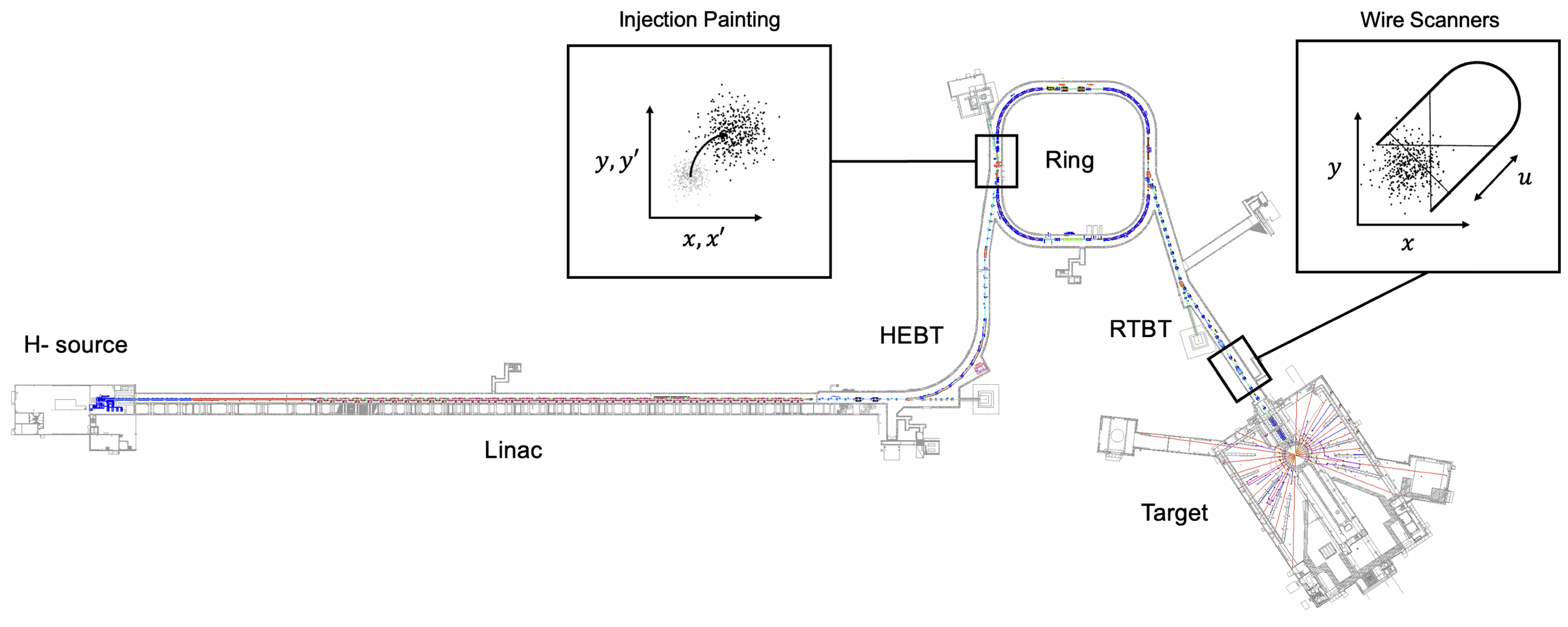
The basic setup is shown in Figure 11. Eight dipole “kicker” magnets control the phase space coordinates at the injection point. Our goal was to program these kicker magnets to trace the correct path in phase space during injection, then measure the accumulated distribution.
One difficulty is that the SNS kicker magnets are fairly weak; they cannot deliver the large angular impulses required for the method. In his simulations, Jeff lowered the energy from 1 GeV to 600 MeV to increase the effective kicker strength (radians per volt). In our experiment, we were only able to lower the energy to 800 MeV.6 So we had to work with smaller angular kicks and, therefore, a smaller beam emittance.7
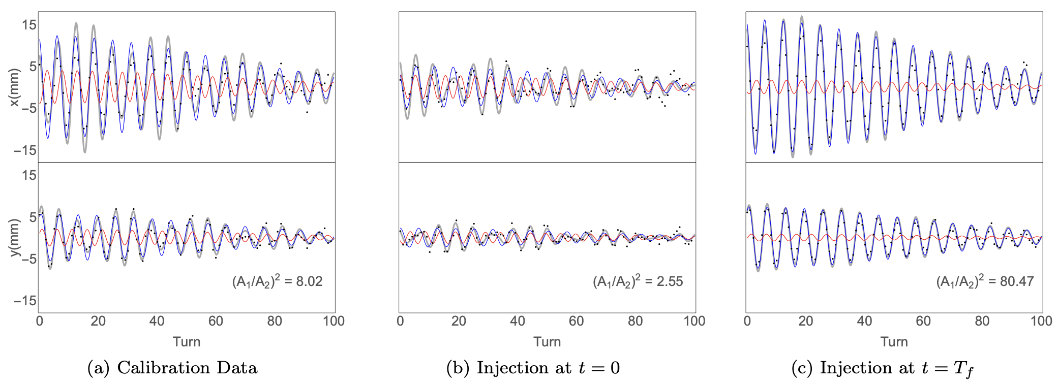
Another difficulty is that we don’t directly control the injection coordinates — we control kicker waveforms. We needed a way to map kicker amplitudes (V) to phase space coordinates (m, rad). We measured the injection coordinates indirectly by injecting a single minipulse into the ring, recording the turn-by-turn centroid position, and then fitting a linear model to the data. The analysis is slightly complicated by the energy distribution in the minipulse, which causes particles to spread around each eigenvector ellipse (recall Figure 2) and eventually eliminates the centroid oscillations. This is called chromatic damping. The damping occurs over about 100 turns, and we have a good model of it, so we just add the damping time as a fit parameter. Repeating the measurement at different kicker amplitudes builds a map from kicker amplitudes to phase space coordinates. Once that’s done, we try to find the kicker amplitudes corresponding to the initial and final injection points.
Figure 12 shows data from one of the many BPMs in the ring. In each figure, the grey curve shows the linear model fit, the blue curve shows the mode-1 component, and the red curve shows the mode-2 component. The left figure shows an initial machine state used for calibration. Notice that both modes contribute to the signal. The middle column shows the start of injection (\(t = 0\)), when the amplitudes should be as small as possible. We did not actually reach zero amplitude, but the amplitudes are smaller than in the other figures; we want to correct this in future experiments. The right figure shows the end of injection (\(t = 1\)). Notice that the first mode frequency dominates over the second, as expected for particles injected along an eigenvector.
After this setup, we used a square-root waveform to connect the initial and final kicker voltages and ran the full beam accumulation over 600 turns. Unlike in the simulation, we can’t directly measure the four-dimensional phase space distribution in the ring. I therefore applied the MENT algorithm to reconstruct the distribution from one-dimensional profiles of the extracted beam. The reconstruction is an inference from incomplete data, so there is some uncertainty in the results, but we’re pretty confident in the major features. (See [10] for details.)
Figure 13 shows the reconstructed distribution in normalized coordinates (Equation 12}, projected onto the two-dimensional phase planes. The second two rows show a simulated distribution.
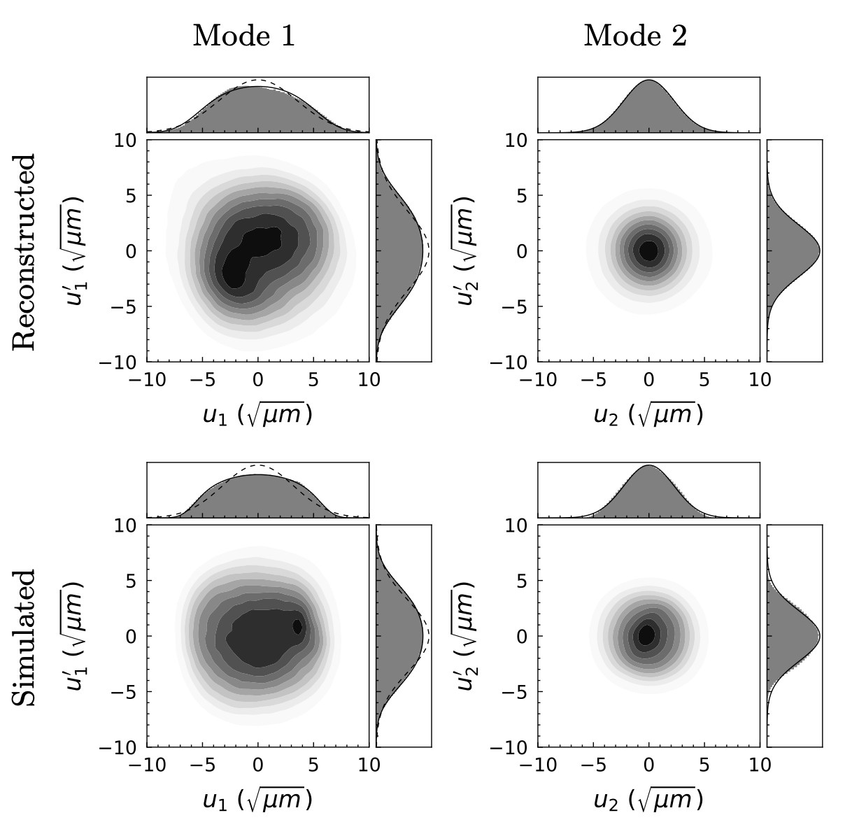
Compare Figure 13 to Figure 4. Ideally, the mode-1 projection would be a uniform disk, and the mode-2 projection would be a small Gaussian blob. While our beam deviates from this ideal case, we do see increased uniformity in the mode-1 projection. The mode-1 emittance is also larger than the mode-2 emittance, giving a ratio \(\varepsilon_1 / \varepsilon_2 = 2.4\). Based on the minipulse size and maximum painting amplitudes, we expected a maximum ratio of 16. We believe that space charge is the primary cause of four-dimensional emittance growth relative to the ideal case. But we also think the emittance growth can be largely reduced in future experiments. (More on that in a second.)
The distribution’s features are qualitatively reproduced in our simulations, though some differences remain. The simulated emittance ratio is 2.3, close to the measured value.
Conclusions and future work
This project had four main parts: (i) connecting the proposed painting scheme to the eigenvector analysis of linear motion, which we now understand well; (ii) programming the kicker waveforms and measuring the injected phase space coordinates; (iii) reconstructing the four-dimensional phase space distribution from one-dimensional measurements; and (iv) comparing the simulated distribution to the reconstruction. In hindsight, it was a lot of work.
Since writing the paper, I’ve been encouraged about the potential to improve our results. I’ve learned a few things from our PIC runs. First, the space charge tune shift was huge in our experiment. Lowering the energy from 1.3 GeV to 0.8 GeV increases the tune shift by a factor of 2.5 based on the inverse scaling of space charge with energy. We also painted a very small beam because of our kicker limitations. I estimate that the tunes shifted well below the integer resonance \(\nu = 6.0\). Subsequent analysis has shown that the beam envelope becomes unstable above ~300 minipulse intensity at the targeted emittance. This instability may have been excited during the early stages of injection, leading to a significant change in beam density. In any case, the dynamics near the integer resonance may be complicated, and I need to spend more time analyzing the simulation to understand what’s going on. The situation can probably be improved by changing the lattice optics, but the immediate next step will be to lower the intensity from 600 to ~200 minipulses. Second, we didn’t account for the effect of space charge on the eigenvectors. Since the experiment, I’ve found that space charge has a strong but predictable effect, and that painting into this modified eigenvector could yield a much larger emittance ratio, perhaps up to \(\varepsilon_1 / \varepsilon_2 \approx 12\). I’ll follow up on this in a future post.
On the simulation side of things, I hope to study the long-term stability of eigen-painted beams and to examine, more generally, four-dimensional phase-space painting as a method of space-charge mitigation.
References
Footnotes
Danilov also proposed Nonlinear Integrable Optics (NIO) [2] and Laser-Assisted Charge Exchange (LACE) [3].↩︎
If we know the covariance is matched to the lattice, but we don’t know the transfer matrix, we can construct the covariance matrix from the eigenvectors in Equation 12↩︎
This is only true in the absence of coherent instabilities…↩︎
It wasn’t labeled ask eigenpainting at that point. We made the explicit connection to eigenvectors later.↩︎
This is an issue with the SNS timing system.↩︎
When we derived eigenpainting, we assumed that the minipulse was much smaller than the final beam. If the beams are comparable in size, the density will be nonuniform. To first order, we can think of the finite-size minipulse as a Gaussian filter which softens the sharp edges of the beam ellipse.↩︎