Maximum entropy for sparse CT

Sparse CT is CT with sparse data, i.e., relatively few projection angles. In medical CT, reducing the number of projection angles reduces the radiation dose given to the patient. This paper has a nice explanation of the problem and a literature review. Medical imaging isn’t my field, but I have worked on CT algorithms in the context of particle accelerators. The problems are pretty much the same, but the number of views is typically much lower in accelerator applications (tens vs. hundreds of views in medical imaging). When there are many views, Fourier methods like Fourier Back Projection (FBP) provide an almost instant high-accuracy reconstruction. But when there aren’t many views, FBP gives poor results and we have to use iterative solvers.

Iterative solvers typically act on the space of image pixels, so for \(N\) pixels we have an \(N\)-dimensional solver. If \(x\) is the image vector and \(y\) is the data vector, tomography involves a linear inverse problem Ax = y to be solved for x, where A is a large sparse matrix. One of the most popular methods to solve sparse linear systems is the Kaczmarz method, also called the algebraic reconstruction technique (ART), and its variants such as SART. More recently, compressed sensing has been used to find solutions that are sparse in some basis by penalizing the \(l_1\) norm of the image vector. There are also approaches using diffusion models that have been trained to sample from CT data sets and act as a type of prior on the space of images.

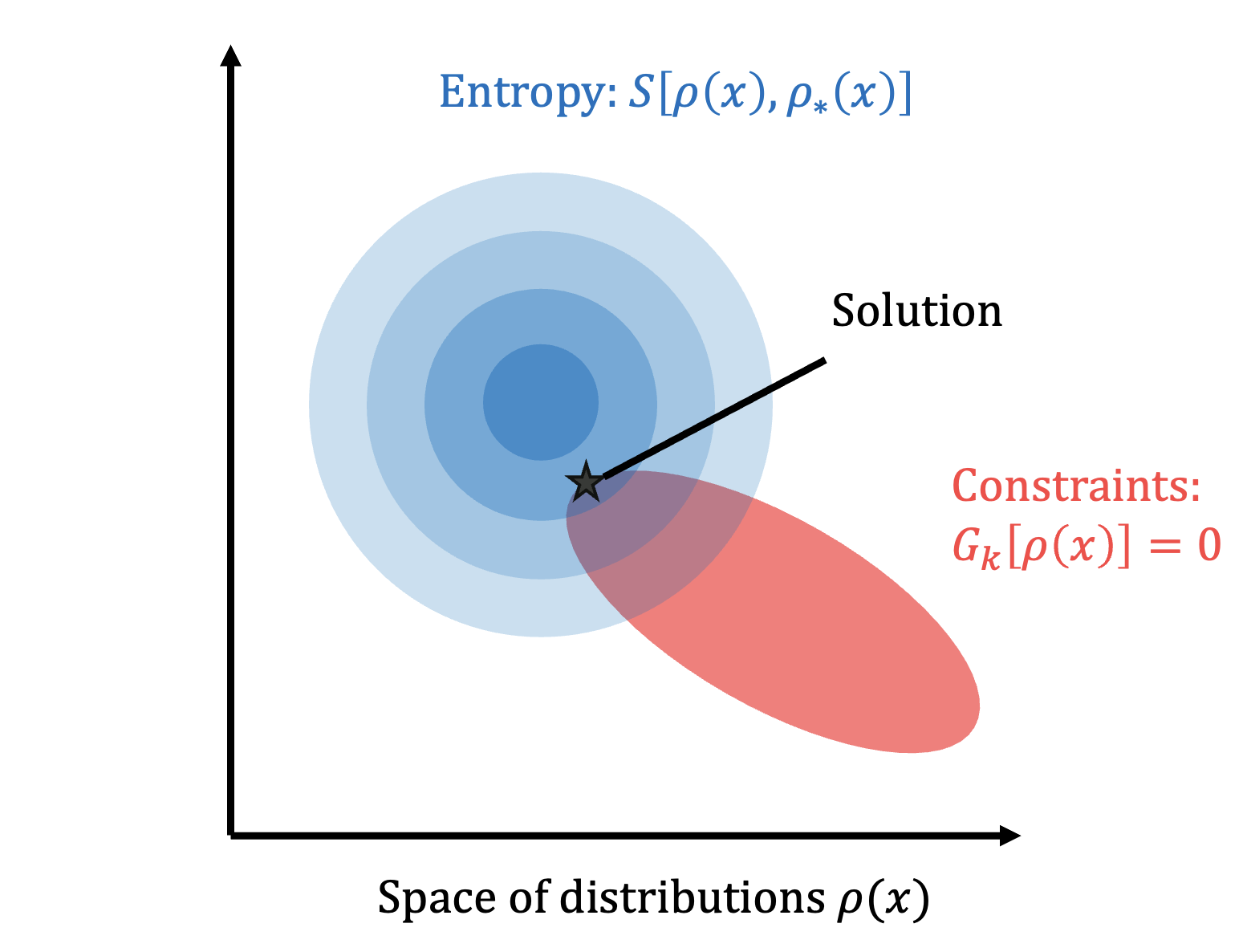
My focus has been on maximum entropy methods, which maximize the relative entropy of the distribution relative subject to the measurement constraints. This method minimizes the complexity of the reconstructed distribution, and is thus perfect for sparse data sets.

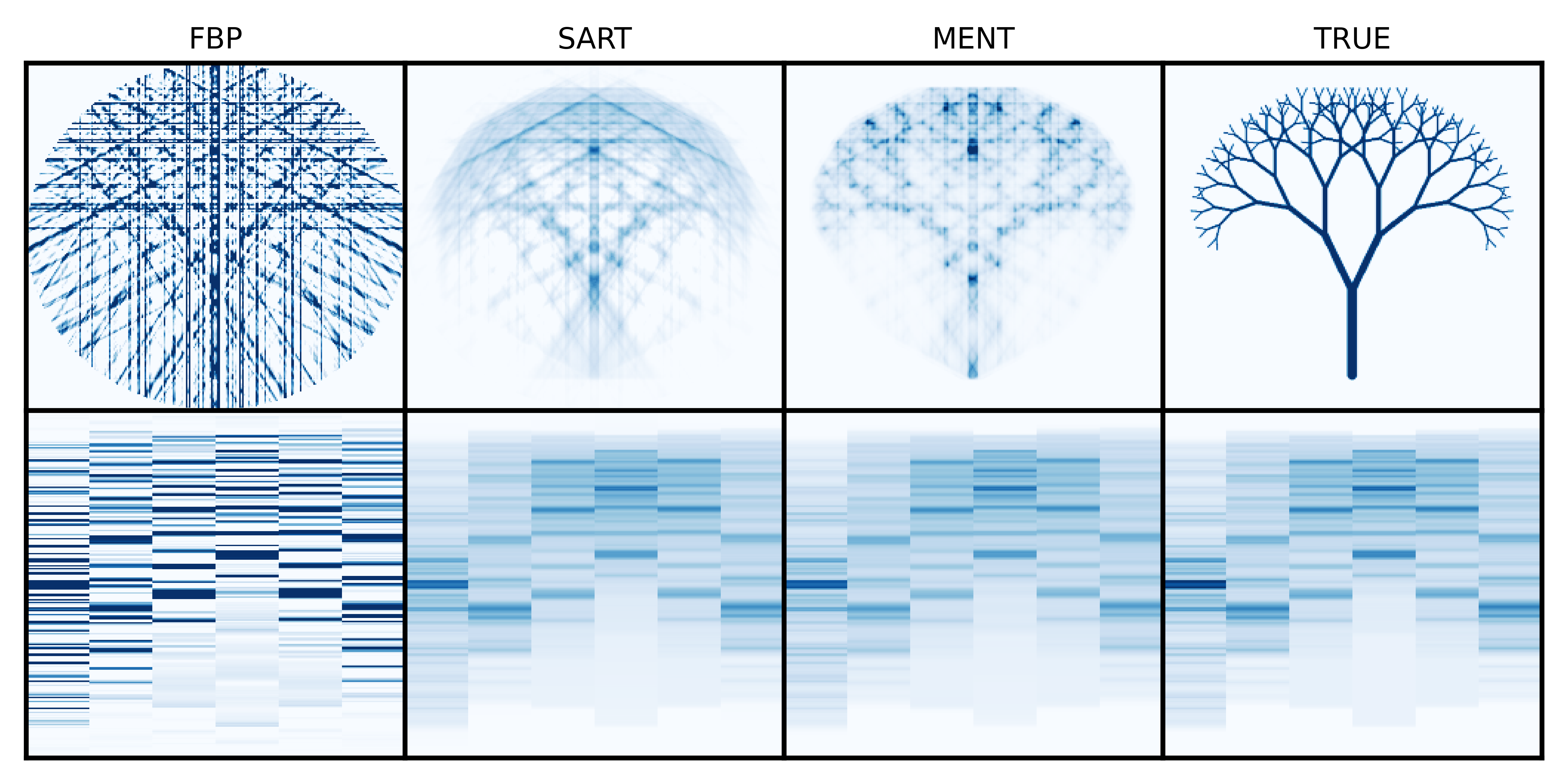
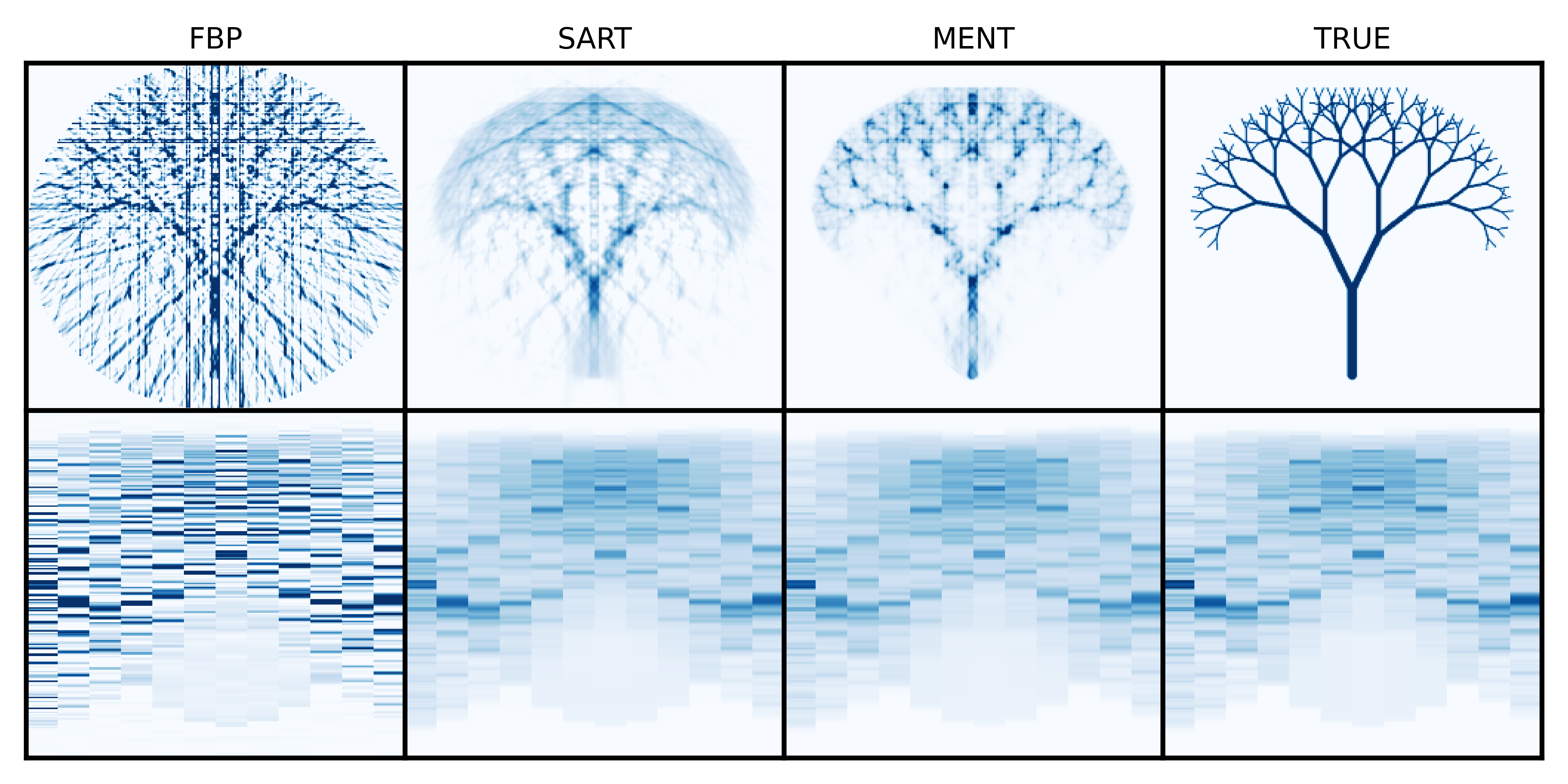
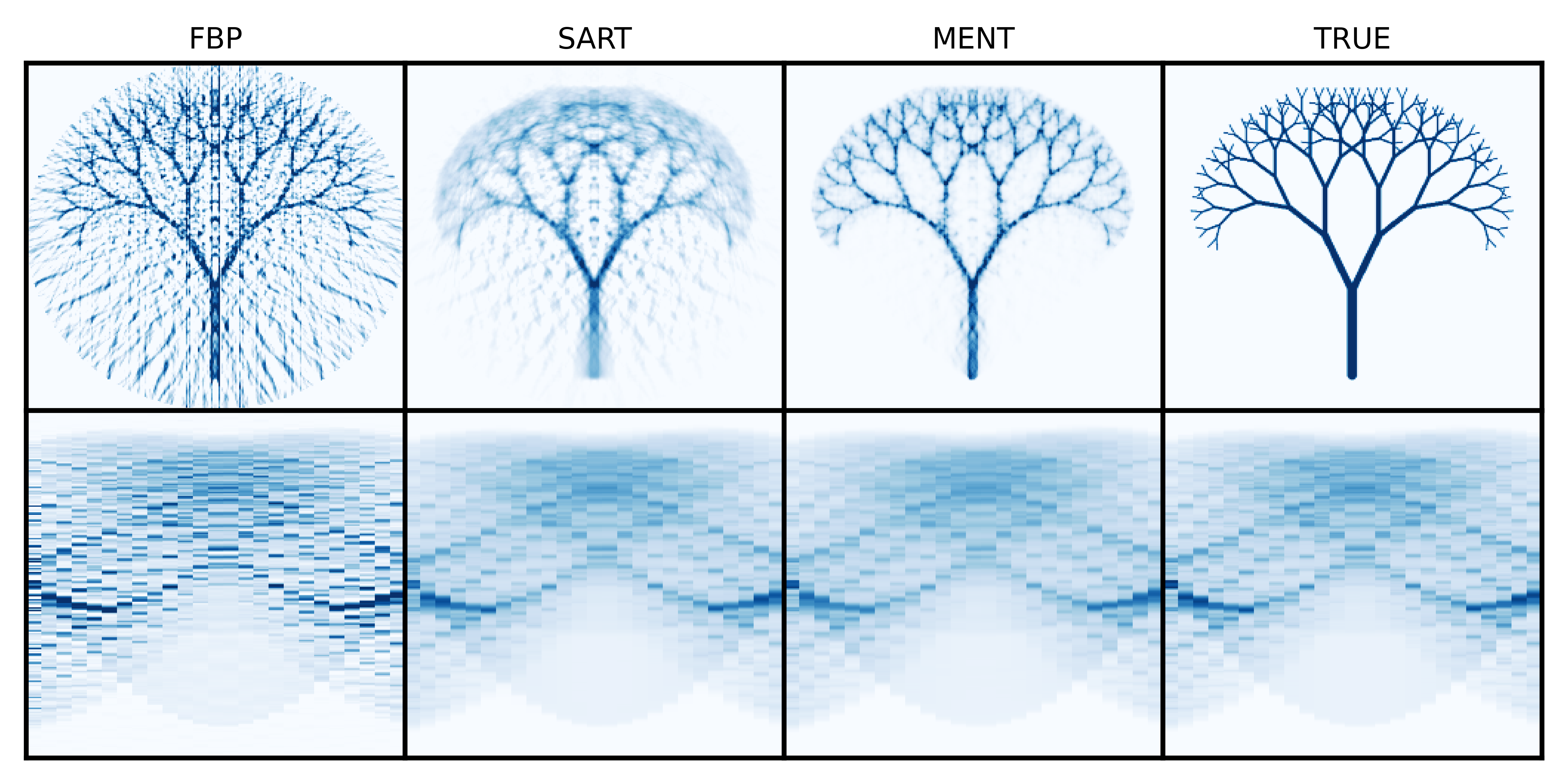
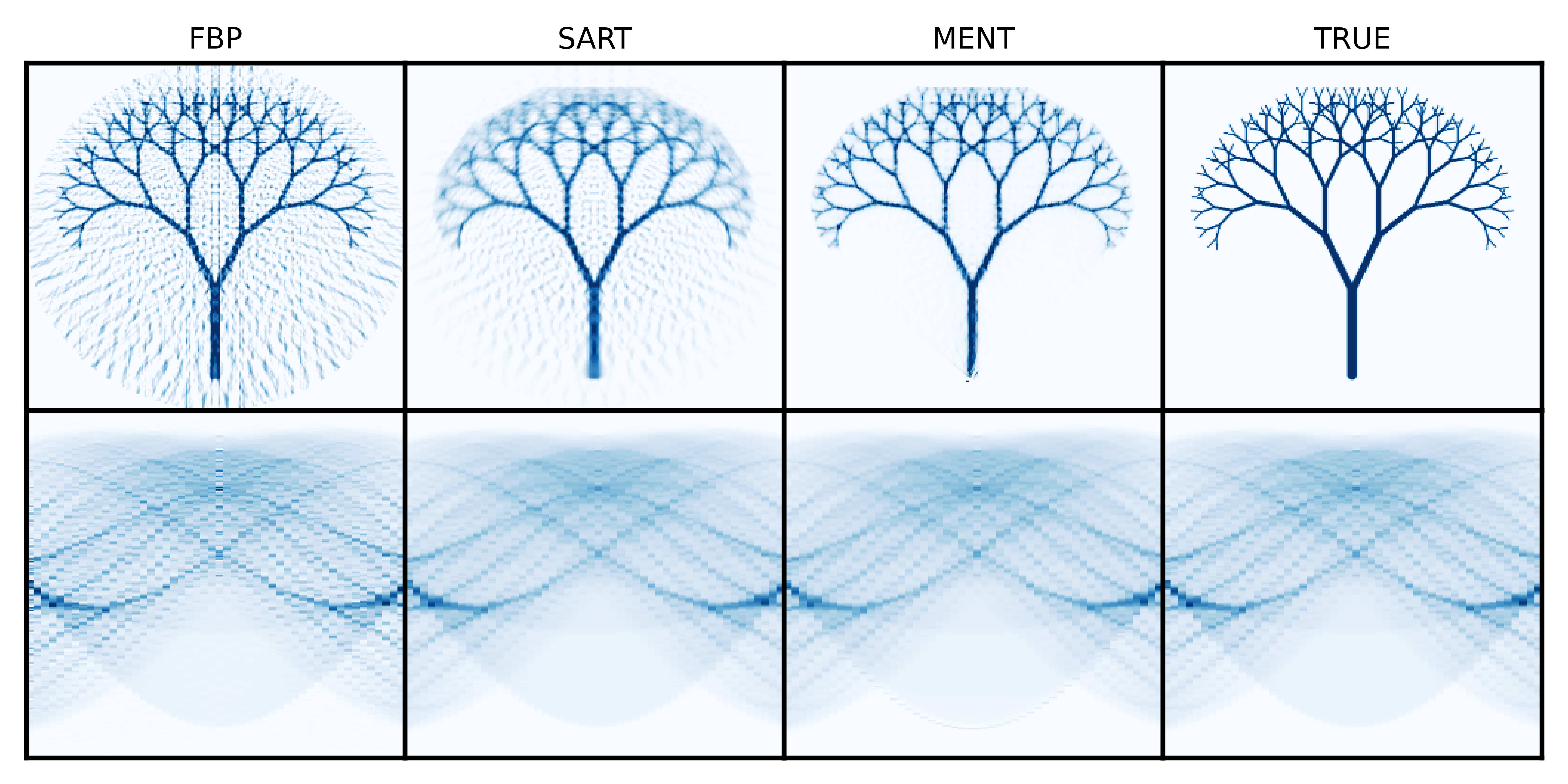
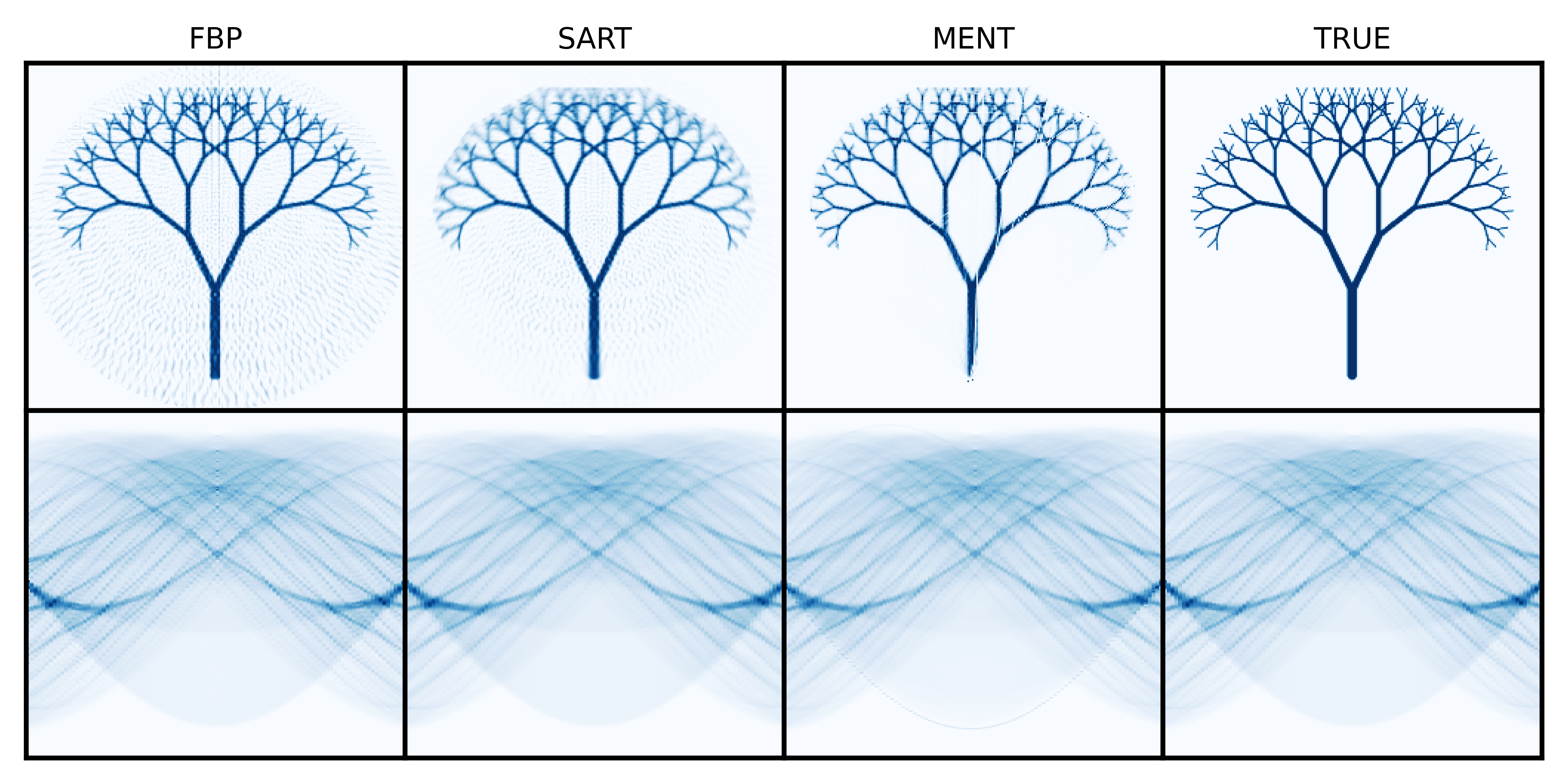
One way to solve the maximum entropy problem is the MENT algorithm, which uses the Lagrange Multiplier method and nonlinear Gass-Seidel iterations to solve the constrained optimization. I’ve recently worked on extending MENT to high-dimensional problems, but I don’t know if I’ve compared it to standard 2D CT solvers. The following is a quick comparison that uses evenly spaced projection angles to reconstruct an image of a tree. I use the MENT package on GitHub and the Radon transform, FBP, and SART algorithms from scikit-image. The results below correspond to 6, 12, 25, 50, and 100 projections.

import numpy as np
import skimage 

def radon_transform(image: np.ndarray, angles: np.ndarray) -> np.ndarray:
    image = np.copy(image)
    image = image.T
    theta = -np.degrees(angles)
    sinogram = skimage.transform.radon(image, theta=theta)
    return sinogram

def rec_fbp(sinogram: np.ndarray, angles: np.ndarray, iterations: int = 1) -> np.ndarray:
    theta = -np.degrees(angles)
    image = skimage.transform.iradon(sinogram, theta=theta)
    return image.T

def rec_sart(sinogram: np.ndarray, angles: np.ndarray, iterations: int = 1) -> np.ndarray:
    theta = -np.degrees(angles)
    image = skimage.transform.iradon_sart(sinogram, theta=theta)
    for _ in range(iterations - 1):
        image = skimage.transform.iradon_sart(sinogram, theta=theta, image=image)
    return image.T

"""Test 2D MENT with high-resolution image."""
import argparse
import os
import time

import numpy as np
import matplotlib.pyplot as plt
import ment  # https://github.com/austin-hoover/ment

from utils import load_image
from utils import rec_fbp
from utils import rec_sart
from utils import radon_transform


plt.rcParams["axes.linewidth"] = 2.0
plt.rcParams["image.cmap"] = "Blues"
plt.rcParams["savefig.dpi"] = 700.0
plt.rcParams["xtick.minor.visible"] = True
plt.rcParams["ytick.minor.visible"] = True


# Arguments
# --------------------------------------------------------------------------------------

parser = argparse.ArgumentParser()
parser.add_argument("--nmeas", type=int, default=25)
parser.add_argument("--iters", type=int, default=5)
parser.add_argument("--lr", type=float, default=0.50)
parser.add_argument("--sart-iters", type=int, default=5)
args = parser.parse_args()


# Setup
# --------------------------------------------------------------------------------------

ndim = 2
nmeas = args.nmeas

output_dir = "outputs"
os.makedirs(output_dir, exist_ok=True)


# Ground truth image
# --------------------------------------------------------------------------------------

res = 512
image_true = load_image(res=res)

xmax = 1.0
grid_edges = 2 * [np.linspace(-xmax, xmax, res + 1)]
grid_coords = [0.5 * (e[:-1] + e[1:]) for e in grid_edges]
grid_points = np.vstack([c.ravel() for c in np.meshgrid(*grid_coords, indexing="ij")]).T


# Forward model
# --------------------------------------------------------------------------------------

angles = np.linspace(0.0, np.pi, args.nmeas, endpoint=False)

transforms = []
for angle in angles:
    matrix = ment.utils.rotation_matrix(angle)
    transform = ment.sim.LinearTransform(matrix)
    transforms.append(transform)


# Training data
# --------------------------------------------------------------------------------------

sinogram = radon_transform(image_true, angles)

projections = []
for j in range(sinogram.shape[1]):
    projection = ment.Histogram1D(
        values=sinogram[:, j],
        coords=grid_coords[0],
        axis=0,
        thresh=0.001,
        thresh_type="frac",
    )
    projection.normalize()
    projections.append([projection])


# Reconstruction model
# --------------------------------------------------------------------------------------

prior = ment.GaussianPrior(ndim=2, scale=10.0)

integration_limits = [[(-xmax, xmax)] for _ in range(nmeas)]
integration_size = image_true.shape[1]

model = ment.MENT(
    ndim=ndim,
    transforms=transforms,
    projections=projections,
    prior=prior,
    sampler=None,
    integration_limits=integration_limits,
    integration_size=integration_size,
    integration_loop=False,
    mode="integrate",
    verbose=0,
)


# Training
# --------------------------------------------------------------------------------------

for iteration in range(args.iters):
    model.gauss_seidel_step(learning_rate=args.lr)


# Plot results
# --------------------------------------------------------------------------------------

# Make dictionary for comparison:
results = {}
for method in ["fbp", "sart", "ment", "true"]:
    results[method] = {}
    for key in ["sinogram", "image"]:
        results[method][key] = None

# TRUE
image_true = image_true.copy()
sinogram_true = radon_transform(image_true, angles)
results["true"]["sinogram"] = sinogram_true.copy()
results["true"]["image"] = image_true.copy()

# MENT
image_pred = model.prob(grid_points).reshape(image_true.shape)
sinogram_pred = radon_transform(image_pred, angles=angles)
results["ment"]["image"] = image_pred.copy()
results["ment"]["sinogram"] = sinogram_pred.copy()

# FBP
image_pred = rec_fbp(sinogram_true, angles)
sinogram_pred = radon_transform(image_pred, angles=angles)
results["fbp"]["image"] = image_pred.copy()
results["fbp"]["sinogram"] = sinogram_pred.copy()

# SART
image_pred = rec_sart(sinogram_true, angles, iterations=args.sart_iters)
sinogram_pred = radon_transform(image_pred, angles=angles)
results["sart"]["image"] = image_pred.copy()
results["sart"]["sinogram"] = sinogram_pred.copy()

# Normalize and scale
for key in ["image", "sinogram"]:
    for name in results:
        results[name][key] /= np.sum(results[name][key])
    for name in results:
        results[name][key] /= np.max(results["true"][key])

# Plot images and sinograms
fig, axs = plt.subplots(ncols=4, nrows=2, figsize=(9.0, 4.5), gridspec_kw=dict(wspace=0, hspace=0), tight_layout=True)
for j, name in enumerate(results):
    for i, key in enumerate(["image", "sinogram"]):
        axs[0, j].pcolormesh(results[name]["image"].T,  vmin=0.0, vmax=1.0)
        axs[1, j].pcolormesh(results[name]["sinogram"], vmin=0.0, vmax=1.0)
    axs[0, j].set_title(name.upper()) 
for ax in axs.flat:
    ax.set_xticks([])
    ax.set_yticks([])
plt.savefig(os.path.join(output_dir, "fig_compare_all.png"), transparent=True)

Observations: (1) Both MENT and SART generate nearly identical sinograms (projections). (2) MENT eliminates all streaking artifacts. (3) MENT is slow but not too slow. The reconstruction with five GS iterations takes a a few seconds when there are fewer projections and up to a minute at the maximum of 100 projections. The speed could be improved using multiprocessing. Note that MENT does not directly deal with the sparse forward matrix. The runtime scales with the square of the number of projections, unfortunately.

It seems like MENT could be a nice algorithm for sparse CT, unless there are other considerations I’m unaware of. I don’t have time to look into this, but I might reach out to someone in the field for their opinion.