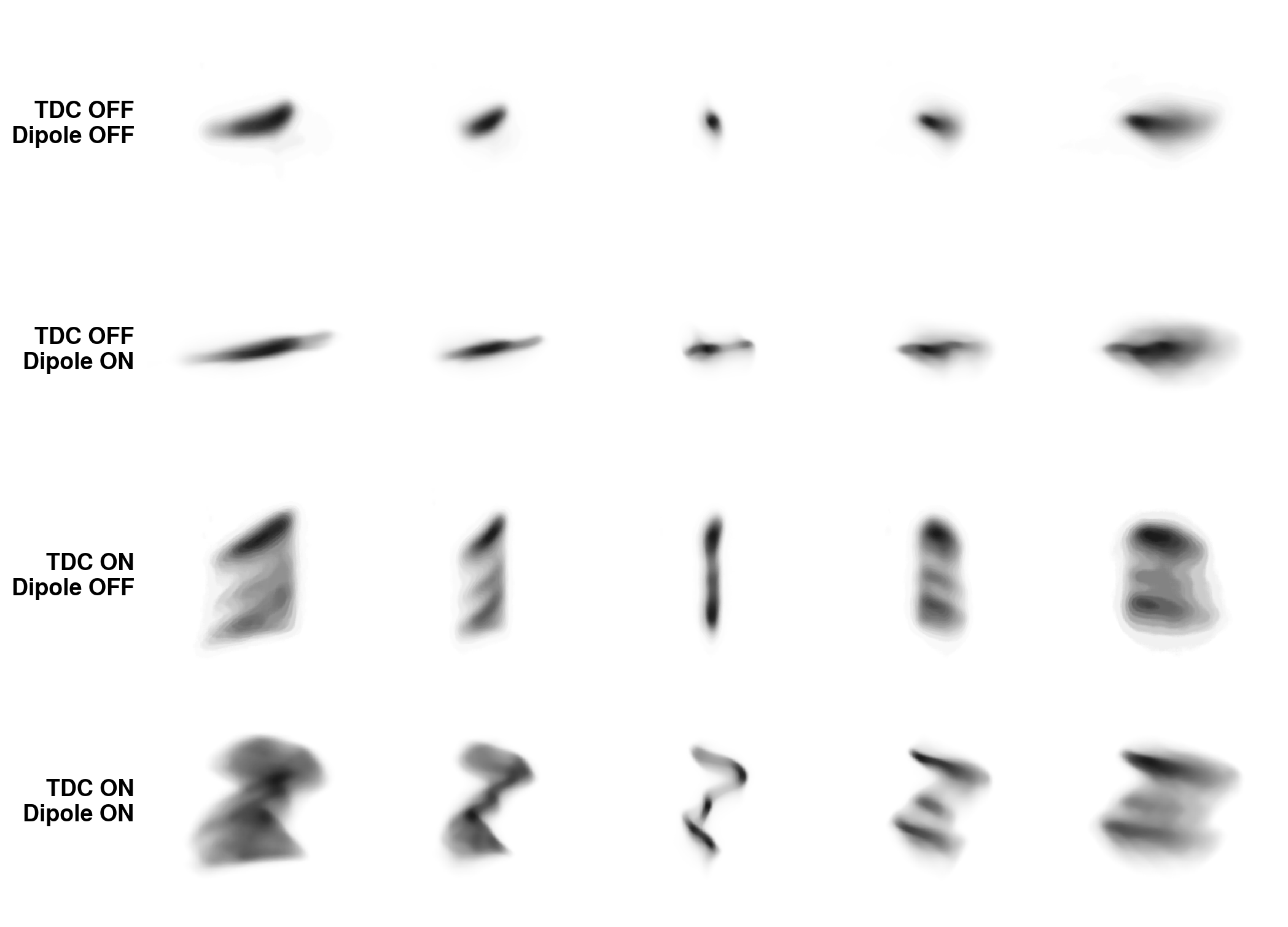
Applying 6D MENT to data
Last year I submitted a paper called N-dimensional maximum-entropy tomography via particle sampling. (See this post.) The idea was to use Markov Chain Monte Carlo (MCMC) sampling techniques to approximate high-dimensional integrals that appear in the MENT algorithm. I demonstrated the method on a toy problem, reconstructing a 6D Gaussian Mixture (GM) distribution from its pairwise projections.
I finally got around to submitting a new version. I added an example where I applied MENT to data from the Argonne Wakefield Accelerator (AWA). The data set is described in this paper by Roussel et al. and is shared in an open-source repository. It contains 36 measured images of an electron beam in the AWA beamline, each with a different set of accelerator parameters.
The accelerator begins with a series of quadrupole magnets, each of which provides linear focusing in one transverse plane (\(x\)) and defocusing in the other plane (\(y\)). The quadrupoles are followed by a transverse deflecting cavity (TDC). The TDC generates a sinusoidal electric field that points mainly along the \(y\) axis. Particles receive a vertical momentum kick dependent on arrival time, rotating the longitudinal coordinate \(z\) into the vertical plane. The TDC is followed by a dipole bend, which couples the horizontal position \(x\) to the longitudinal momentum \(p_z\) because of momentum dispersion. There are two beamlines after the dipole so that the beam can be measured with the dipole on or off. Scanning the quadrupoles constrains the 4D transverse phase space density \(\rho(x, p_x, y, p_y)\). Quadrupole scans were repeated with the TDC turned on/off, and then with the dipole turned on/off, generating different transverse-longitudinal correlations in the distribution at the measurement screen. A full 6D reconstruction is necessary to fit the data.
The authors used a differential simulation to propagate particles through the accelerator and a differentiable kernel density estimator to compute the \(x\)-\(y\) projections. The differentiable forward model enables gradient-based optimization of the phase space distribution. A generative model was used to represent the distribution, and the model parameters were varied to minimize the pixel-wise error between measured and simulated images. This is called Generative Phase Space Reconstruction (GPSR). Very cool method!
It’s straightforward to apply MENT to arbitrary problems using this GitHub implementation. The key step is to create a list of functions that transform input phase space coordinates to output phase space coordinates, where the coordinates are passed as NumPy arrays. The transformations do not need to be differentiable. In this case, I just wrote a wrapper function that takes a NumPy array, transforms the NumPy array using the Bmad-X accelerator (the differentiable simulation), and then converts back to NumPy at the end. One complication is that it’s best to estimate the covariance matrix of the unknown phase space distribution. This is mostly for the MCMC sampling algorithm, which performs best on “round” distributions, i.e., distributions with roughly the same variance in every direction and no linear correlations between variables. I mention a few strategies to estimate the covariance matrix in the paper. In this example, I just assumed a known covariance matrix which I obtained from the previous GPSR fit.
I used the Metropolis-Hastings (MH) algorithm to sample particles from the MENT distribution function. I chose MH because it does not require a differentiable target distribution and is simple to code. We start with a set of points at random locations \(x_t\) in the phase space. Then we sample another point \(x_*\) from a jumping distribution \(q\), which we take to be a Gaussian. The new point is accepted or rejected according to the following procedure: \[\begin{equation} {x}_{t + 1} = \begin{cases} {x}_* & \text{if}\ r \leq \pi({x}_* | {x}_t), \\ {x}_t & \text{otherwise}, \end{cases} \end{equation}\] where \[\begin{equation} \pi({x}_* | {x}_t) = \text{min} \left( 1, \frac{ \rho({x}_*) }{ \rho({x}_t) } \frac{ q({x}_t | {x}_*) }{ q({x}_* | {x}_t) } \right), \end{equation}\] where \(r \in [0, 1]\) is a random number.
MH converges to the target distribution in the long run, but its performance is highly dependent on the jumping distribution. Too wide, and most points will be rejected; too narrow, and it will take forever to explore the space. Although there’s a whole literature on tuning and diagnosing MCMC, I just tuned the width of the Gaussian jumping distribution until the acceptance rate was ~0.25-0.5 and checked that the projections/distribution didn’t look too strange. I sampled around \(5 \times 10^5\) particles with 500-1000 chains, and all chains gave pretty much the same result, so I was fairly confident that the chains converged. Sampling this huge number of particles can be pretty fast using a vectorized MCMC implementation.
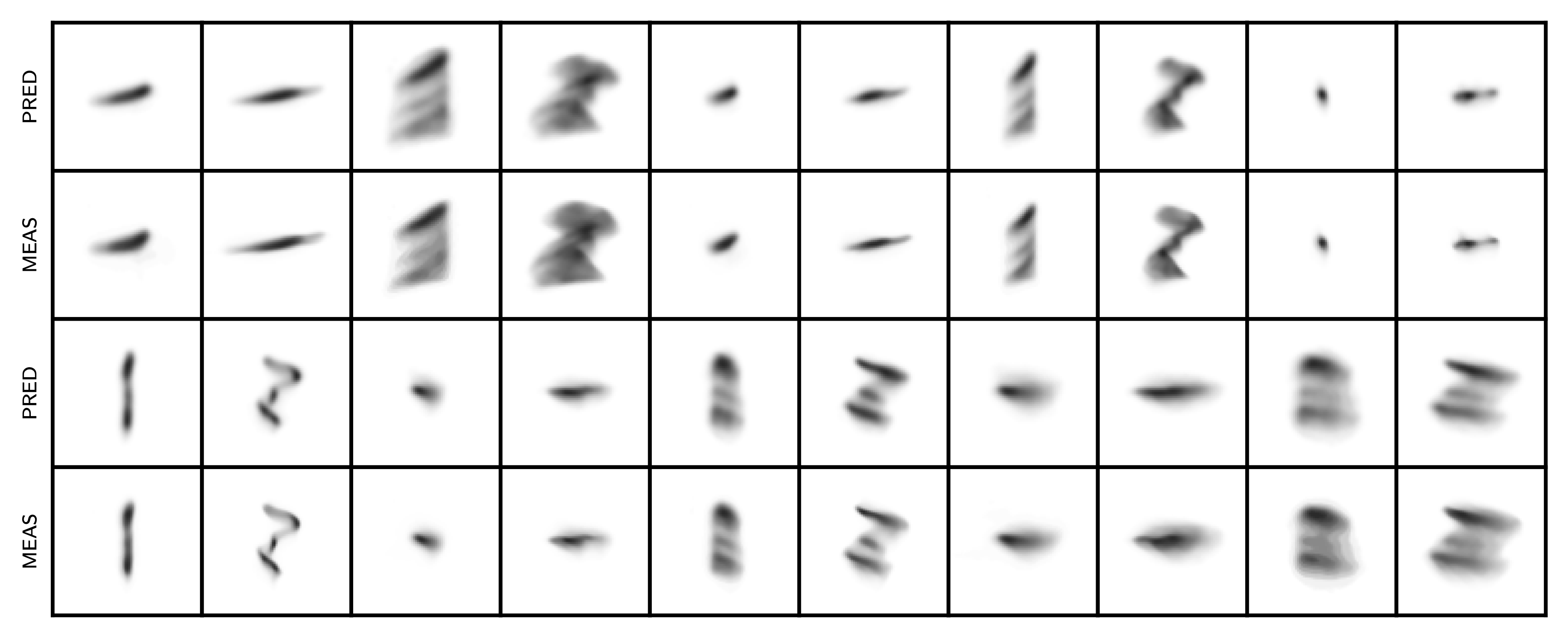
Here are the measured vs. simulated projections of the 6D distribution after a few MENT iterations:
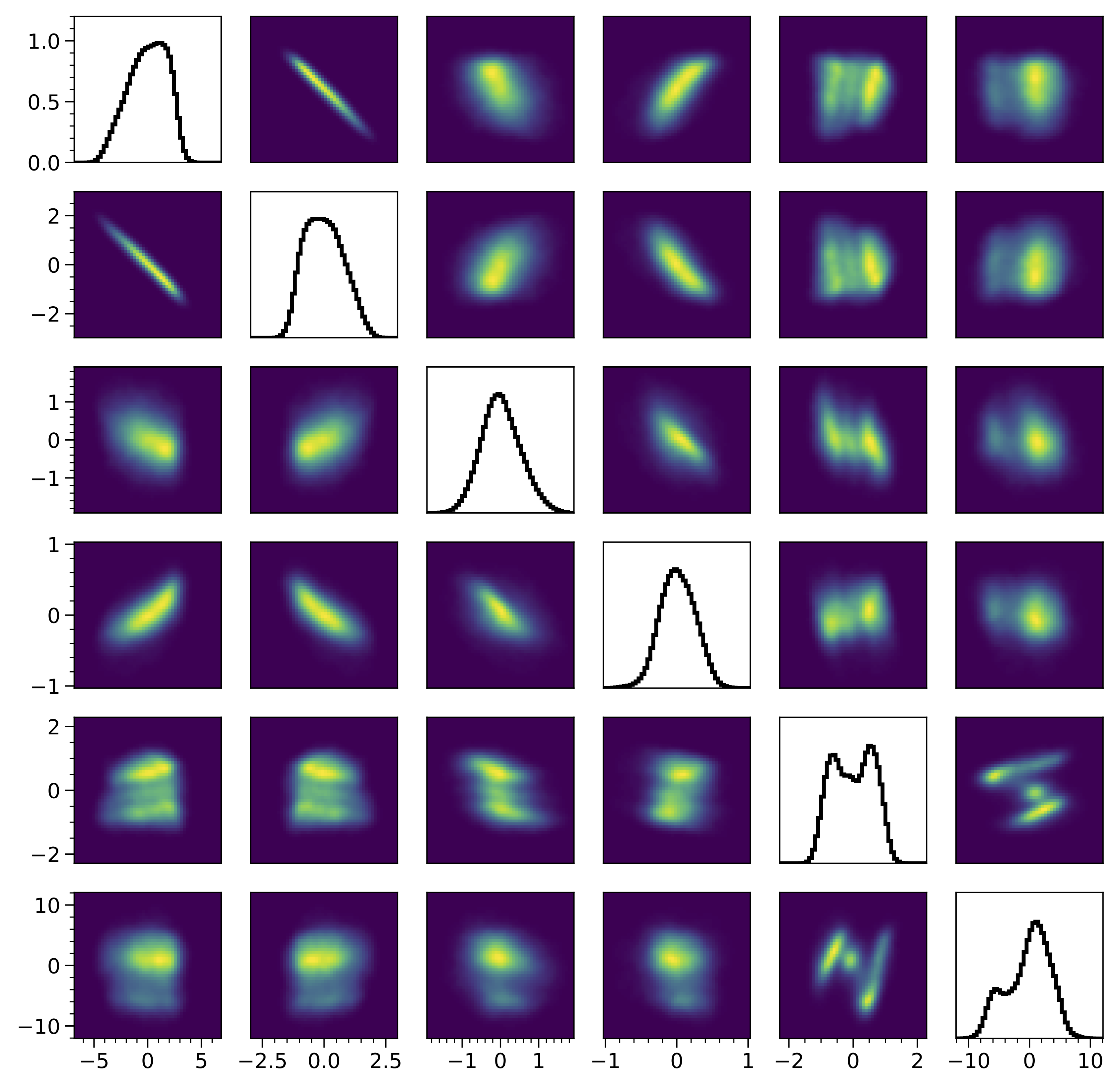
Not bad! I don’t see any major errors. Here are the 1D and 2D marginal projections of the reconstructed 6D MENT distribution compared to GPSR:
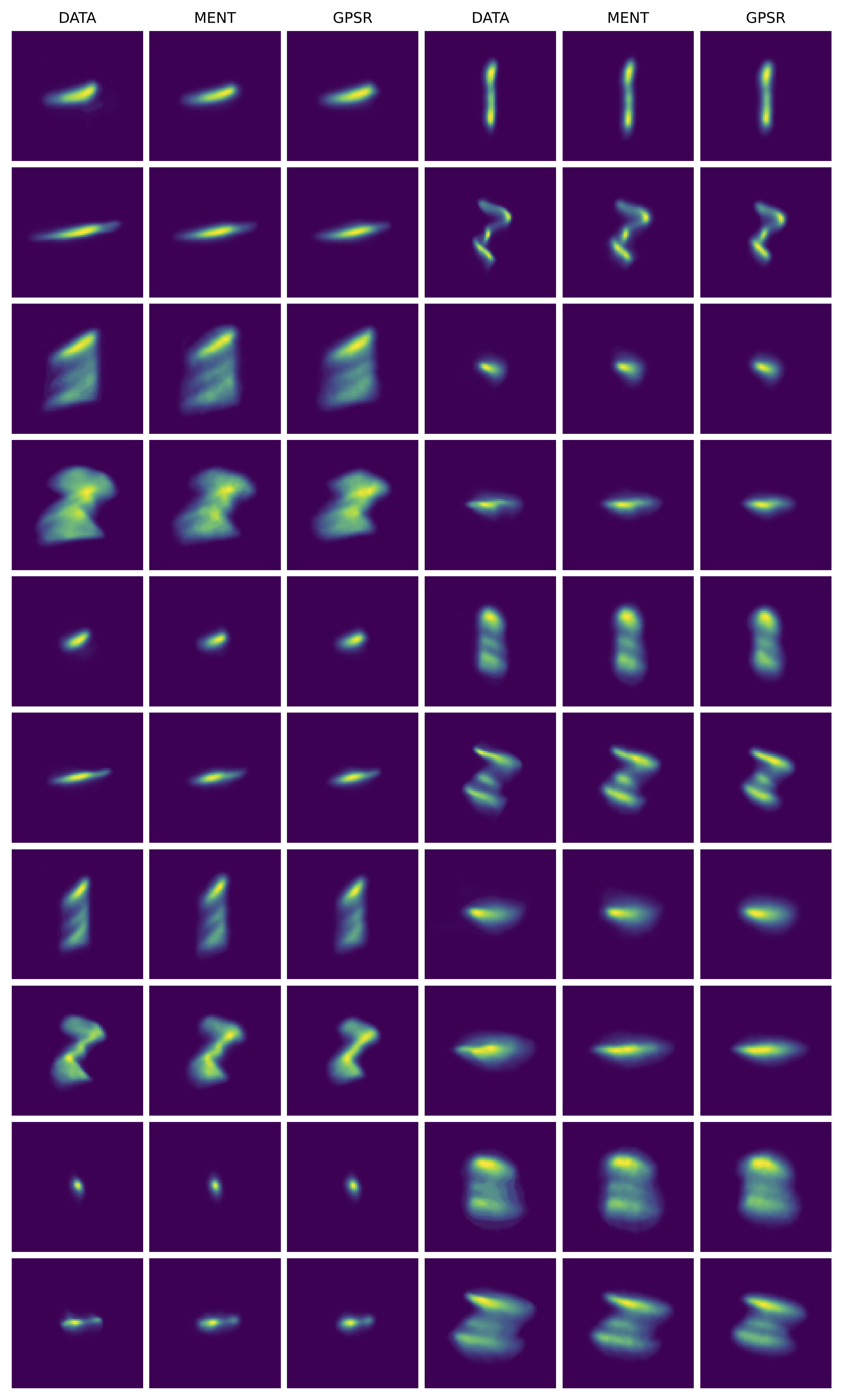
The plots look similar, with the biggest differences in the longitudinal projections, where MENT is smoother. This is some evidence that the problem is well-constrained. The fit errors are small for both models. Here are blurred histograms of 90,000 particles sampled from the MENT and GPSR reconstructions compared to the measured histograms.
I know the MCMC algorithm is not perfect, so I’m not completely convinced that all features in the MENT distribution are suggested by the data. In other words, the entropy may be slightly lower than maximum due to unconverged MCMC chains. The longitudinal distribution is very thin, which I would expect to give MH trouble. However, the distribution matches the data and has a slightly higher entropy than the GPSR reconstruction, so I think I got reasonably close to the entropy maximum. There’s room to explore other sampling methods or improvements to MH.


