Four-dimensional phase space tomography from one-dimensional measurements of a hadron beam
An older post explained how I used MENT-Flow to reconstruct the four-dimensional phase space density of a beam in the SNS ring. I’ve since improved the reconstruction. First, I found a bug that was setting the beam energy to 1 GeV instead of the correct value of 0.8 GeV. Second, I switched from MENT-Flow to MENT. After making these changes, I reproduced the measured beam profiles almost perfectly. I’ve written up these results in a paper which is under review at PRAB.
The paper isn’t really about the reconstruction algorithm; it’s more about the experimental design and uncertainty quantification needed to trust the results. For instance, it wasn’t clear how many one-dimensional projections we needed to constrain the four-dimensional density.
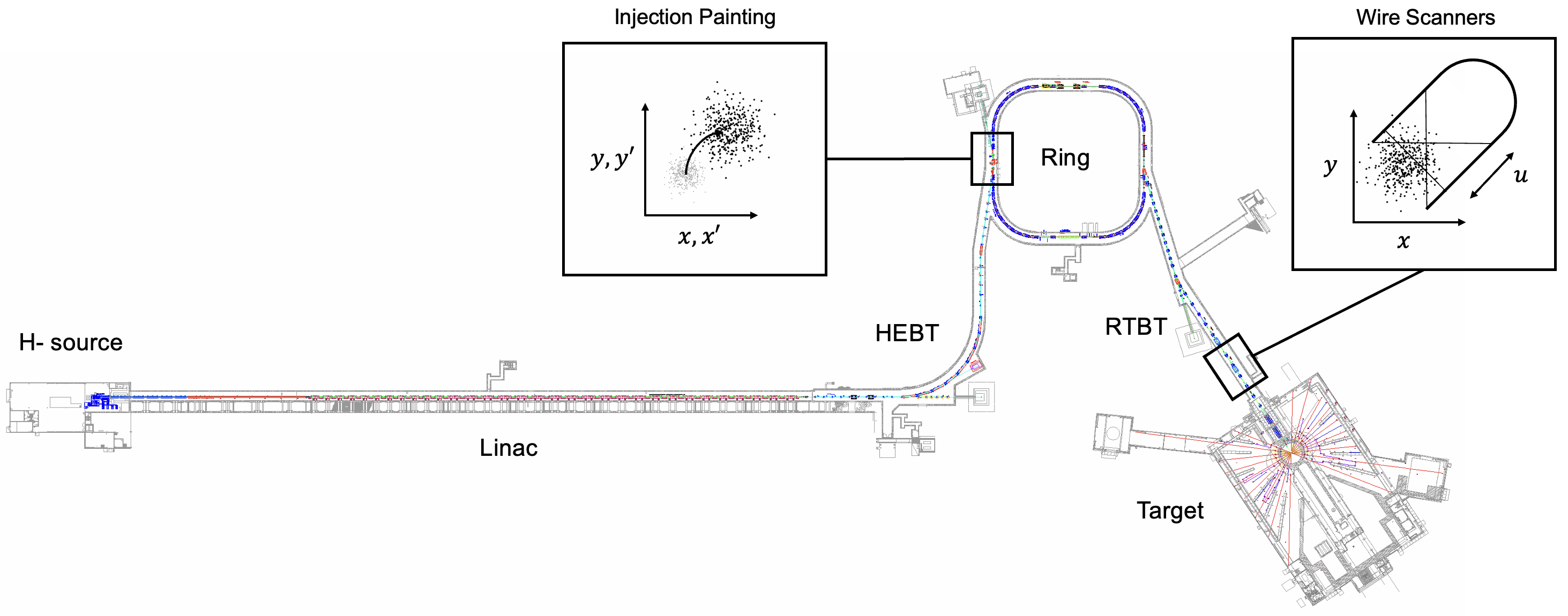
We performed our experiment at the Spallation Neutron Source (SNS) accelerator. The SNS generates high-power proton pulses via multiturn charge-exchange injection from a linac into an accumulator ring. After all \(10^{14}\) protons are accumulated, they’re extracted and sent to the spallation target to make neutrons. We measured the beam in the RTBT (Ring Target Beam Transport) section shown in Figure 1.
The beam intensity and energy preclude the use of screens to measure the two-dimensional beam density. Instead, the SNS has a set of four wire scanners. Each wire scanner has a horizontal, diagonal, and vertical wire that sweeps across the beam. By recording the secondary electron emission from the wire, we can measure the particle density as a function of position. We end up with three signals per wire scanner: \(\{ f(x), f(y), f(u) \}\), where \(u = (x - y) / \sqrt(2)\) is the diagonal axis. The wire scanners run in parallel, generating twelve profiles on each scan.
Each signal is a one-dimensional projection of the four-dimensional phase space distribution \(f(x, x', y, y')\), where \(x'\) and \(y'\) are the momentum coordinates. In an older study, I found that we could use the variance of each signal to nail down the \(4 \times 4\) covariance matrix \(\Sigma\). Reconstructing the full distribution is a natural next step.
A key finding in that older study was that the nominal optics lead to an ill-conditioned least-squares problem when computing the covariance matrix. I solved this by adding another set of optics. There isn’t much wiggle room in the wire scanner region (due to shared quadrupole power supplies and beam size constraints), but I found another working point that led to a better-conditioned problem. In our experiment, we measured the beam with the nominal optics, modified optics, and one additional set of optics, generating 36 profiles.
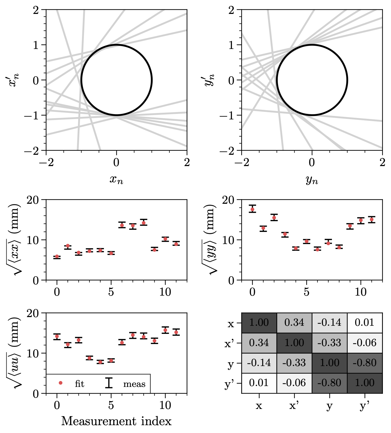
I started by fitting the covariance matrix to the measured signal variances (\(\langle xx \rangle, \langle yy \rangle, \langle uu \rangle\)). Figure 2 shows a tight fit to the data. Using standard least-squares error propagation, I estimated a low sensitivity to errors.
Next, I used MENT to reconstruct the distribution. MENT updates a prior \(f_*(x, x', y, y')\) to a posterior \(f(x, x', y, y')\) by maximizing the entropy of \(f\) relative to \(f_*\). This ensures the posterior is as simple as possible relative to the prior. A uniform prior often makes sense, but we’ve already estimated the covariance matrix from the least-squares fit, and we don’t want to ignore this information. One could imagine starting from a uniform prior and running MENT with the measured covariance matrix as a constraint. The result is a Gaussian distribution. So I used a Gaussian prior with the measured covariance matrix.
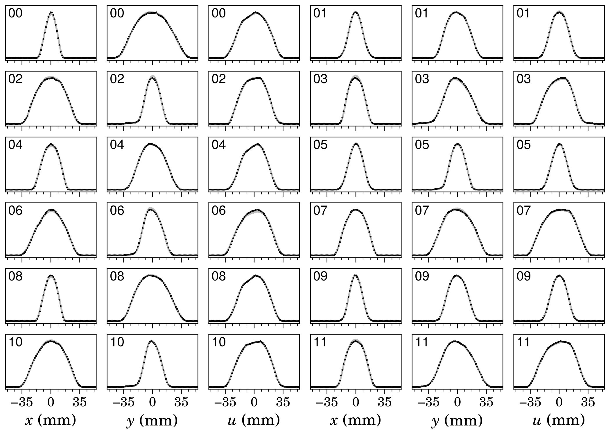
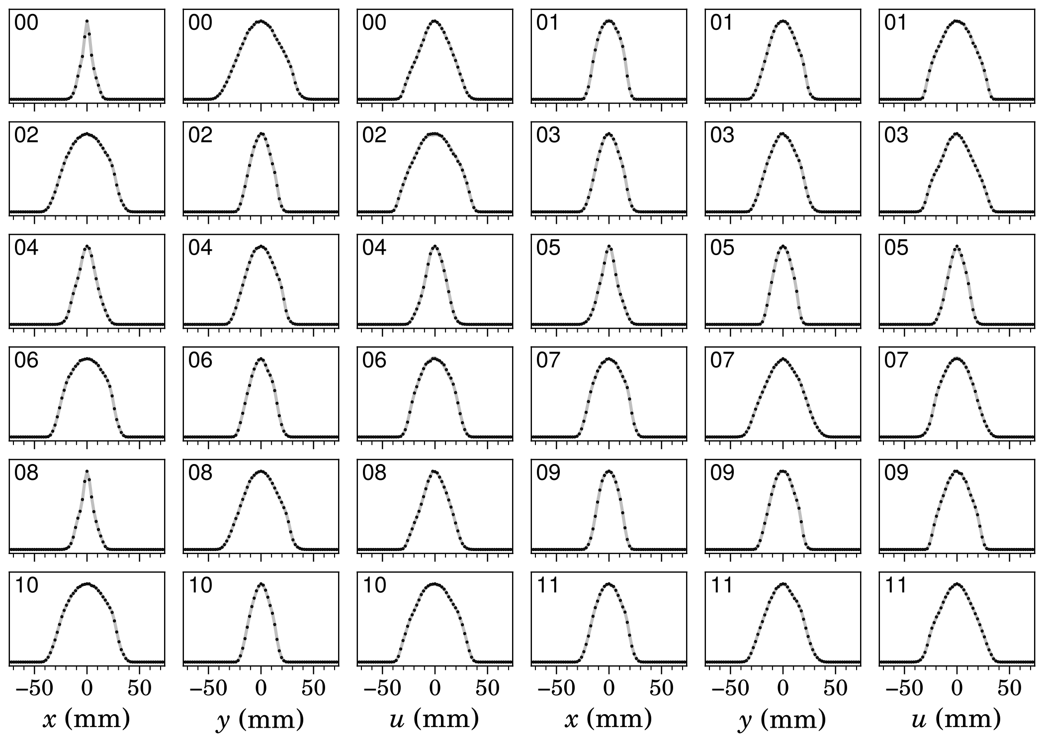
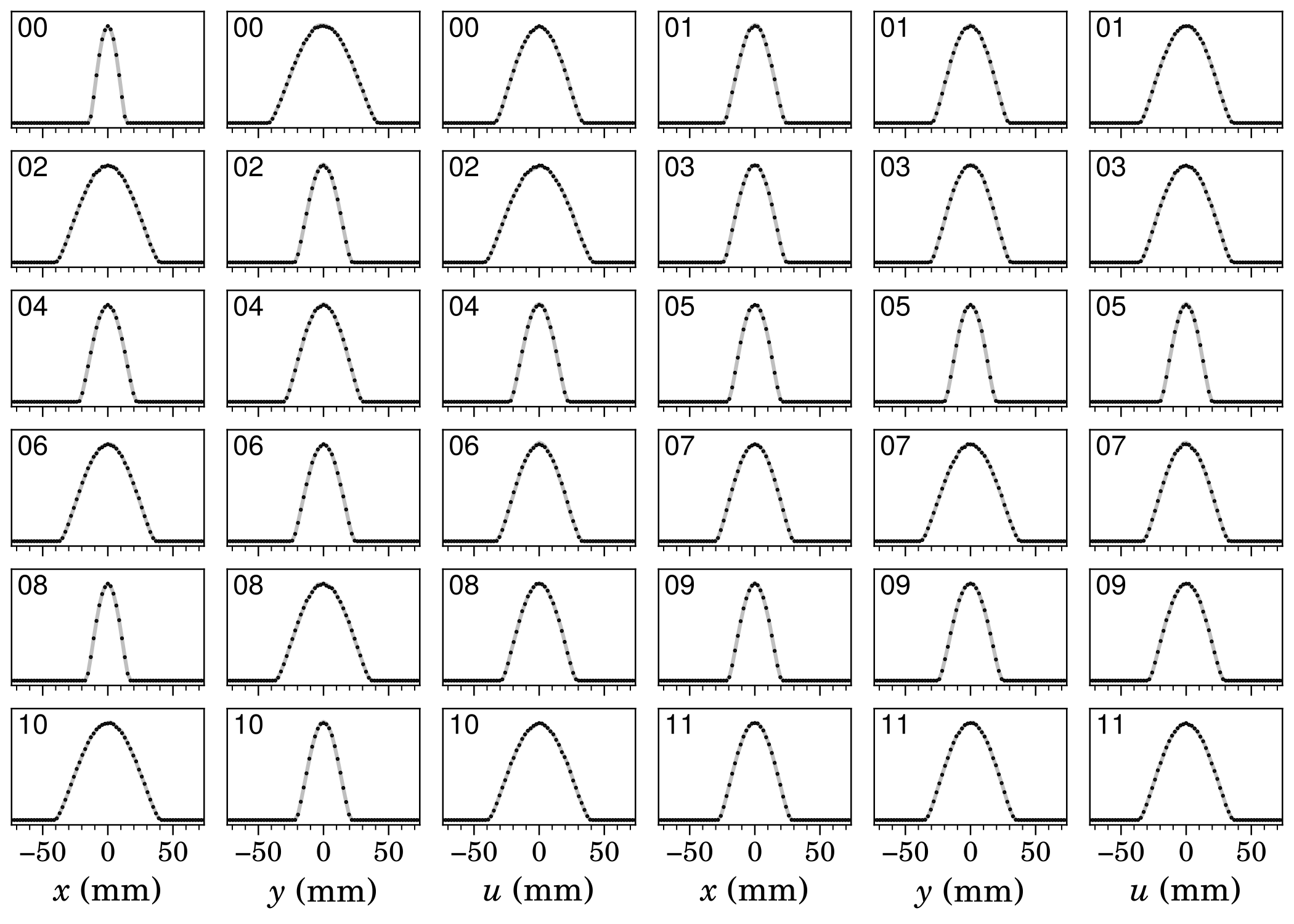
Here are the reconstruction results. First, the measured profiles (black points) compared to the simulated/predicted profiles:
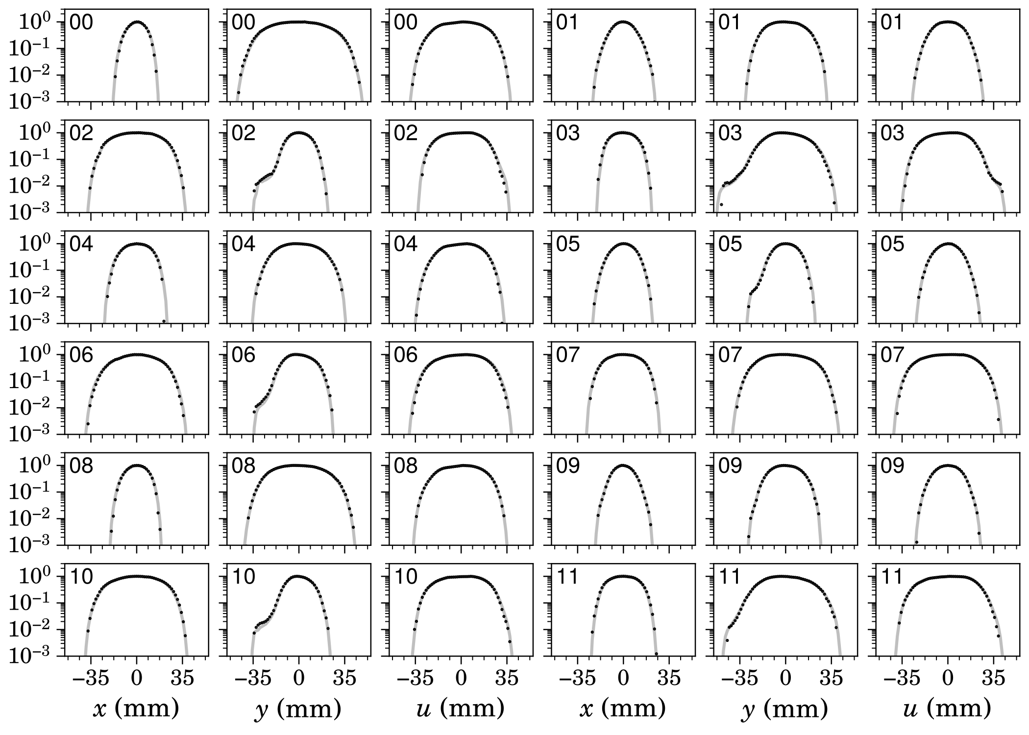
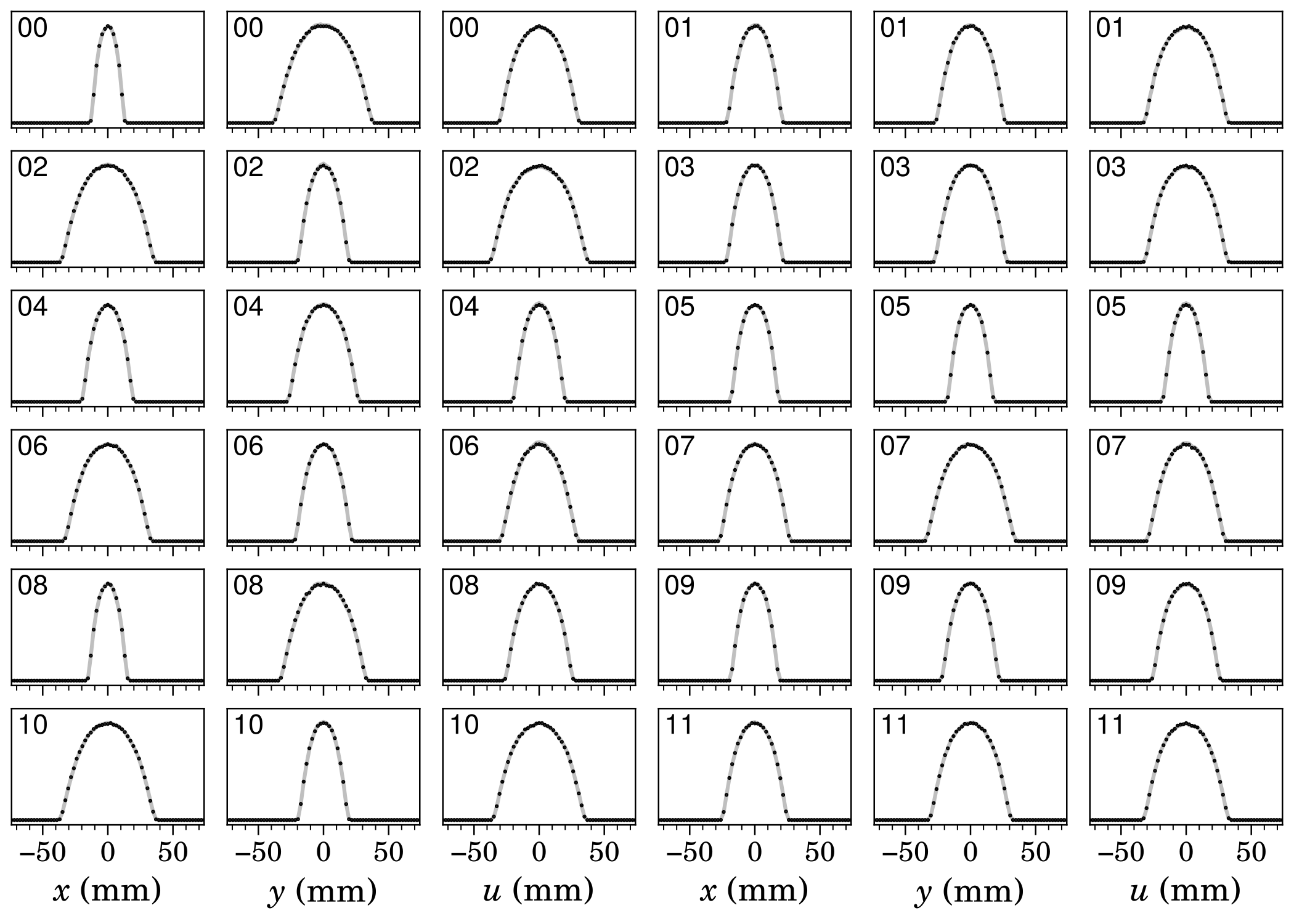
Perfect agreement. The log-scale plots show agreement in low-density regions as well:
I’m not sure what’s causing the shoulders in the vertical (\(y\)) profiles; it might be cross-talk between wires. But this is an encouraging result. It means we might be able to study halo formation in the ring by improving the wire scanner dynamic range.
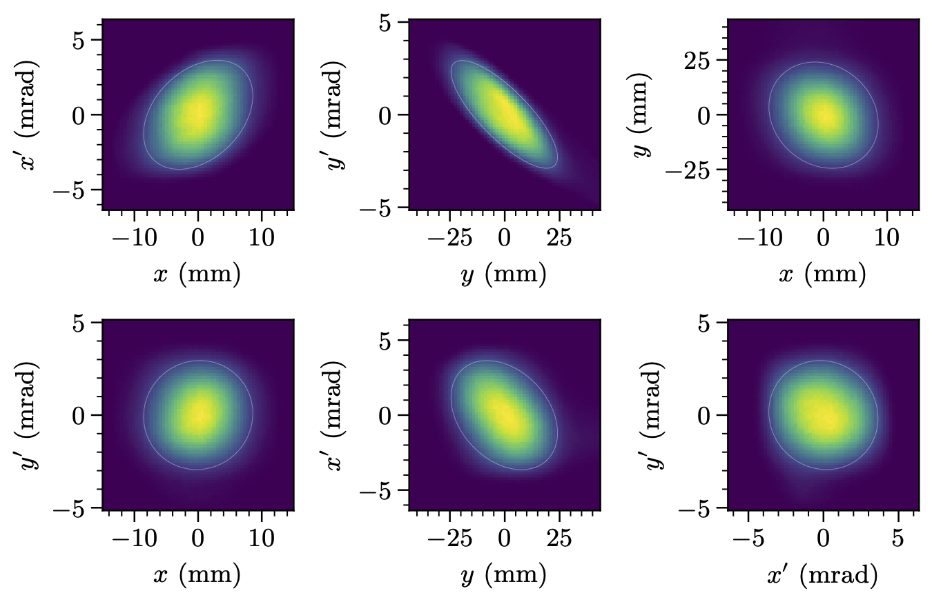
Here are the 2D projections of the 4D distribution that generated those profiles:
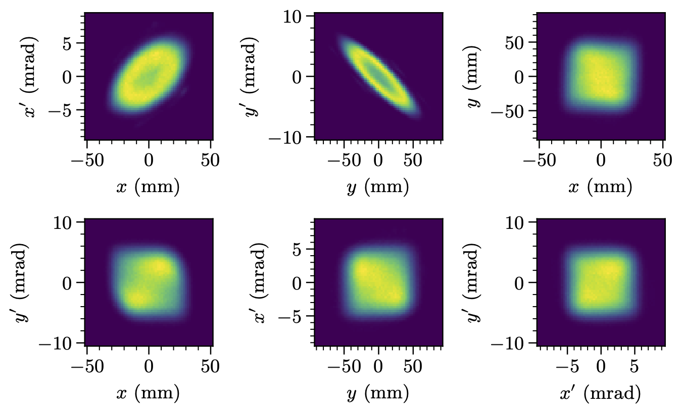
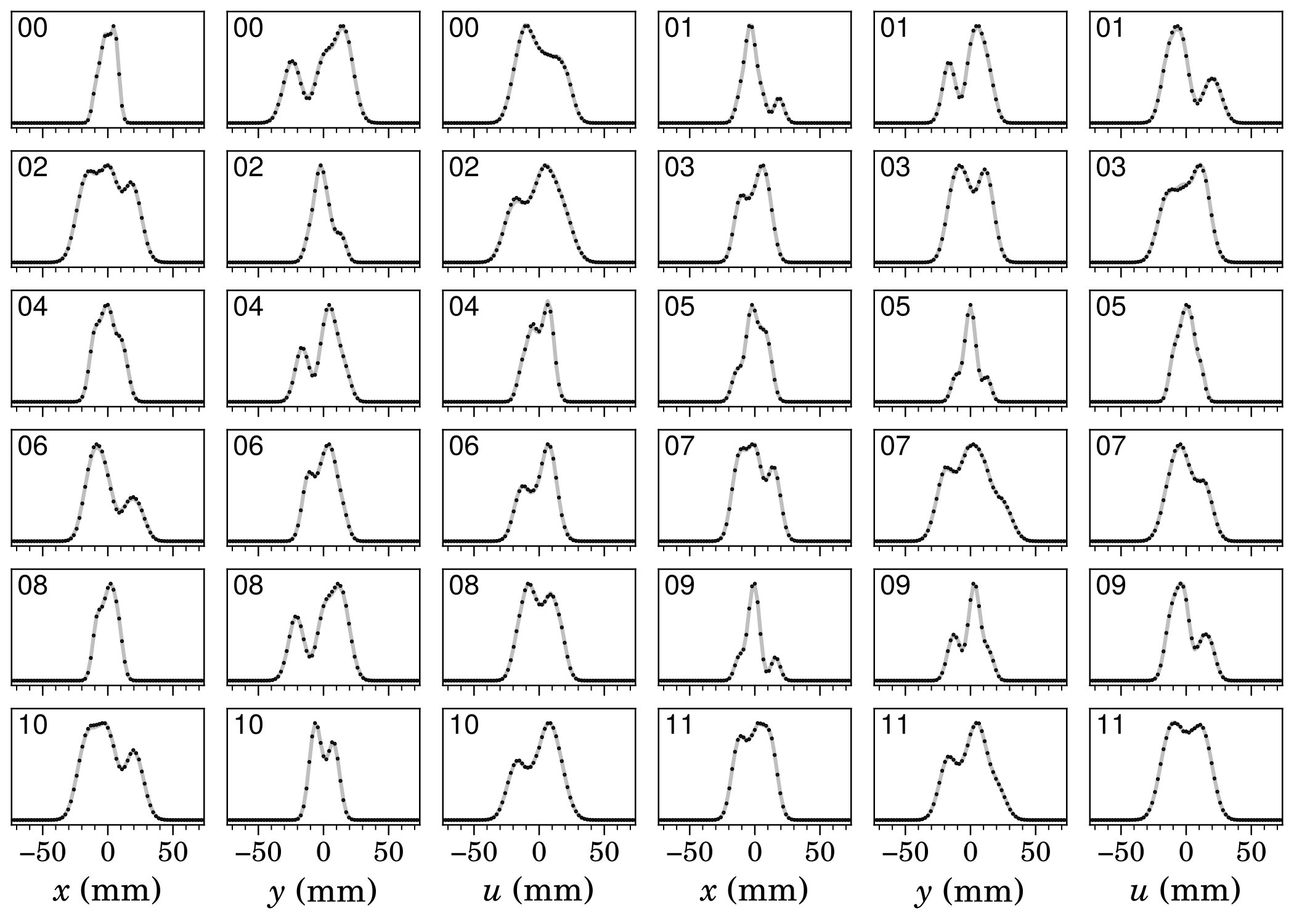
I didn’t say much about this figure in the paper because I was focused on the measurement, not the physics. But note that running the same measurement with a different injection painting scheme yields a much different result (Figure 6). In both cases, the reconstructed distribution is close to what we expected based on simulations.
Should we trust these results? There are many possible errors in the accelerator and measurement model, but we think our modeling errors are quite small. The remaining uncertainty is due to the inverse nature of the reconstruction problem. The measurements render some distributions more likely than others, but they do not identify a unique distribution. An ideal reconstruction algorithm would somehow report the spread of distributions compatible with the measurements. No such algorithm exists at the moment.
Thus I followed the strategy of several other papers: simulate the reconstruction. I used four different initial distributions. The first is the result of a beam physics simulation, so it’s somewhat realistic. The second is a superposition of Gaussian blobs. The third is a “Waterbag” distribution, which has a uniform density inside the unit ball. The fourth is a “Hollow” distribution, which is a hollowed-out version of the Waterbag. Here are the results:
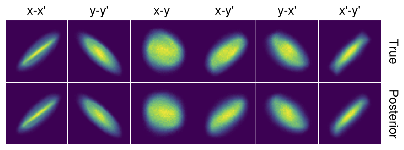
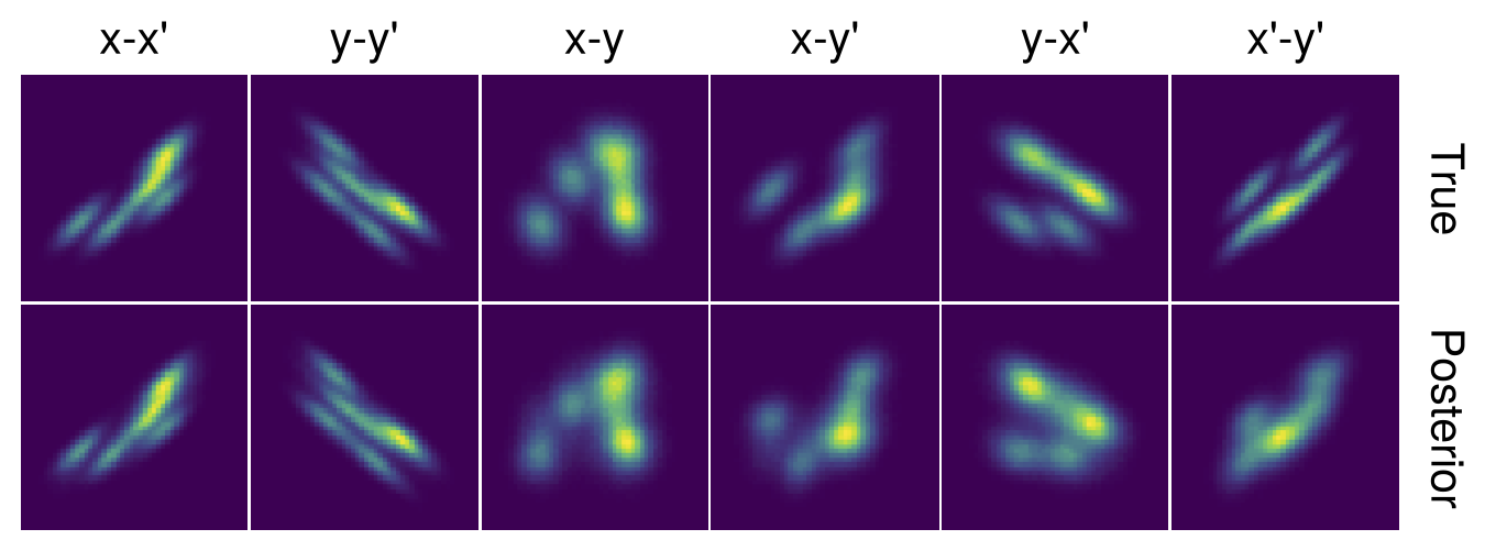
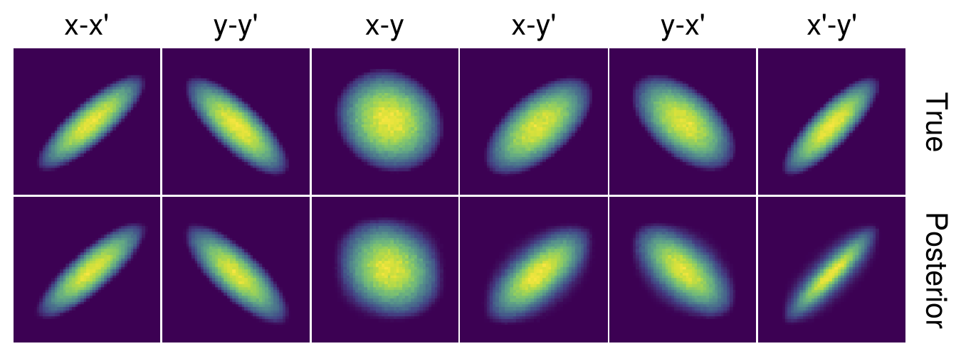
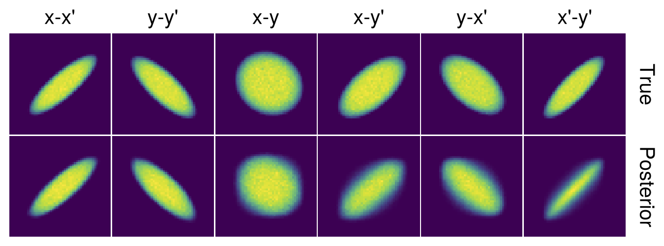
It looks like most 2D features are captured by the MENT distribution. That’s good news for our experiments: 2D features tell us a lot about the beam. There’s more uncertainty in the cross-plane projections, such as \(x\)-\(y\) and \(x'\)-\(y'\), but the uncertainty isn’t enormous.
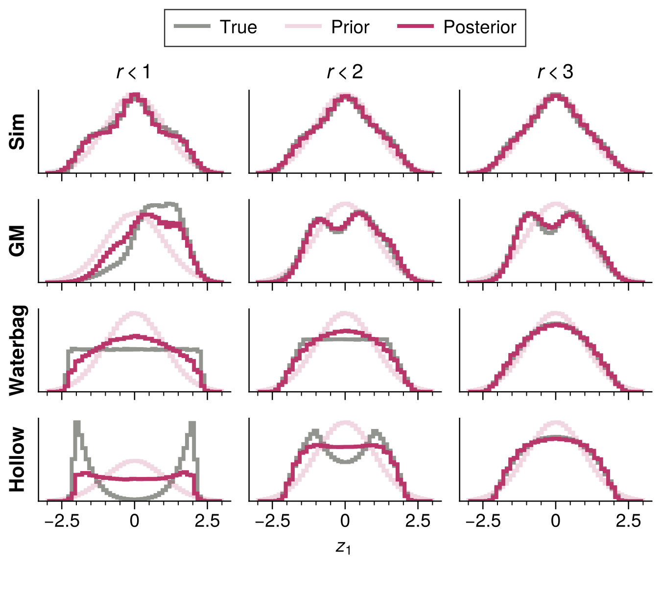
A closer look shows that the internal 4D structure is incorrect for the Waterbag and Hollow distributions. See Figure 7, which shows the 1D projections within a 3D ball in the unplotted coordinates. As the ball shrinks, we approach a 1D slice through the 4D density. You can see that the MENT posterior is uniform, not hollow. Note that both distributions match the data exactly.
The failure to capture the hollow core is somewhat expected from previous studies here, here, and here. Low-dimensional projections average over multiple dimensions and easily hide “holes” in the high-dimensional distribution. There is also a good reason why the MENT posterior is not hollow: the prior is a Gaussian, so MENT will flatten the Gaussian just until the measurements match the data, but no more. In other words, a hollow distribution is very far from the prior.
I concluded that four-dimensional tomography can be useful in real accelerators when only one-dimensional measurements are available. The reconstruction seems reliable for our purposes, as beams are unlikely to be hollow in the SNS ring. Additional constraints or prior information would be needed to reconstruct arbitrary four-dimensional distributions.
I think this method will be useful for benchmarking accelerator physics codes. By extracting the beam on different turns, we can measure the distribution as a function of time: \(f(x, x', y, y', t)\) and compare to the model predictions.
