The impact of phase space correlations on the beam dynamics in linear accelerators
Almost one year ago, CERN hosted the “68th ICFA Advanced Beam Dynamics Workshop on High-Intensity and High-Brightness Hadron Beams”, also known as “HB”. I gave a talk on our work at the SNS Beam Test Facility (BTF). I intended to share that work on this blog, but never got around to it. Better late than never:
The initial beam
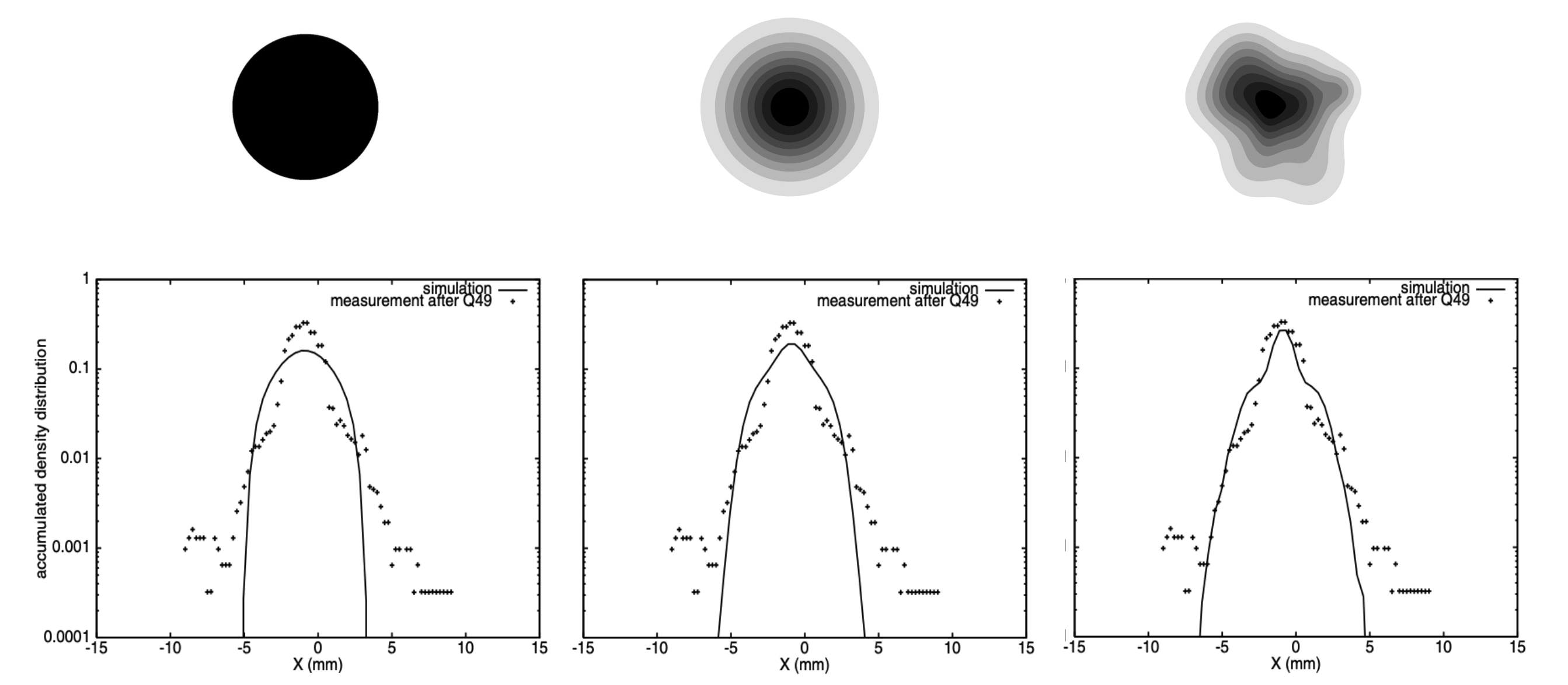
I usually start these talks by reviewing the LEDA (Low Energy Test Accelerator) experiment at Los Alamos National Laboratory [1]. LEDA was a proton source followed by 50 quadrupole magnets arranged in an alternating focus-defocus pattern (FODO). A series of experiments recorded the one-dimensional particle distribution at the end of the accelerator for different sets of quadrupole strengths (optics). In some cases, simulations reproduced the measurements in regions of high particle density, i.e., the beam core. But no simulation reproduced the low-density “tails” or “halo”.
Halo formation is driven by space charge (electric forces between particles). Thus, the discrepancies might have been due to an inaccurate initial distribution in 6D phase space. (They only estimated second-order moments.) On the other hand, errors in the accelerator model might have been to blame. Reproducing halo-level features requires modeling a delicate interplay between applied and self-generated fields.
At the BTF, we’re trying to improve on LEDA’s results. Our primary advantage is a suite of novel phase space diagnostics. One of these diagnostics images the 6D phase space distribution at the beginning of the lattice [3]; another diagnostic measures the beam halo in 2D phase space at the end of the lattice [4]. In the first half of my postdoc, I focused on measurements of the distribution at both locations; see conference reports here and here. We observed major differences between our predictions and measurements. One culprit may have been the paperclip layout of the beamline: bending 180 degrees generated dispersion, and we were unsure if we were modeling the dipole magnets correctly. In any case, linacs do not typically bend, so we upgraded the BTF to a new straight layout. This took several months.
During the upgrade, I examined a question that could be partially answered by computer simulations: How important is the initial 6D phase space structure? In other words, if we ignore correlations between some dimensions, how will this affect the beam dynamics? An easy way to answer this question is to use the measured 6D distribution. However, 6D measurements currently have low resolution (\(\approx 10^6\) points) and low dynamic range (\(\approx 10^1\)); it’s unclear if these values are sufficient to predict halo-level features.
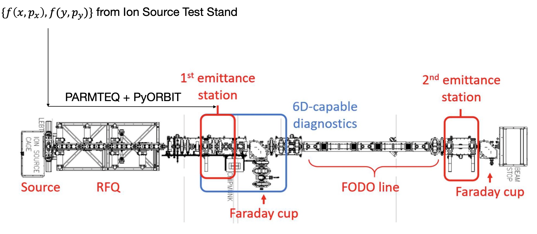
There’s another way to generate the initial beam which avoids direct 6D measurements. The initial beam is not really the initial beam; it’s the beam at the location labeled “First Emittance Station” in Figure 2.
The beam emerges from the source as a continuous stream of ions. The RFQ (Radio Frequency Quadrupole) accelerates the beam to 2.5 MeV and converts the continuous stream to a train of bunches. Before the RFQ, the longitudinal distribution is spatially uniform with a tiny energy spread; thus, defining the initial beam would only require a 4D (transverse) phase space measurement. However, we would then need to simulate the journey through the RFQ, which involves complex dynamics over hundreds of focusing periods with strong space charge. So, we opted for the more difficult 6D measurement after the RFQ.
Still, we could try this approach. We don’t have any diagnostics before the RFQ (there’s no room), but we do have 2D diagnostics at a dedicated Ion Source Test Stand. The ion source is different than the one in BTF, but it should produce a similar distribution. We took some old measurement data of a 50 mA beam in the Ion Source Test Stand and tracked it through the RFQ. The RFQ code (PARMTEQ) predicted a 42 mA beam current, but the real RFQ generated 26 mA. That’s a huge unexplained discrepancy! We’re still unsure what caused this because we can’t peer inside the RFQ. Unphased, we artificially changed the beam current to 26 mA in the simulation and tracked it to the first measurement station.
PARMTEQ vs. reality
The PARMTEQ simulations generate a fully correlated 6D bunch without a direct measurement. The tradeoff is that we’re unsure how realistic this distribution is. We know PARMTEQ gets the basic physics correct, but the model contains various approximations, such as an assumed cylindrical symmetry when solving the Poisson equation. The only way to check is via direct measurements.
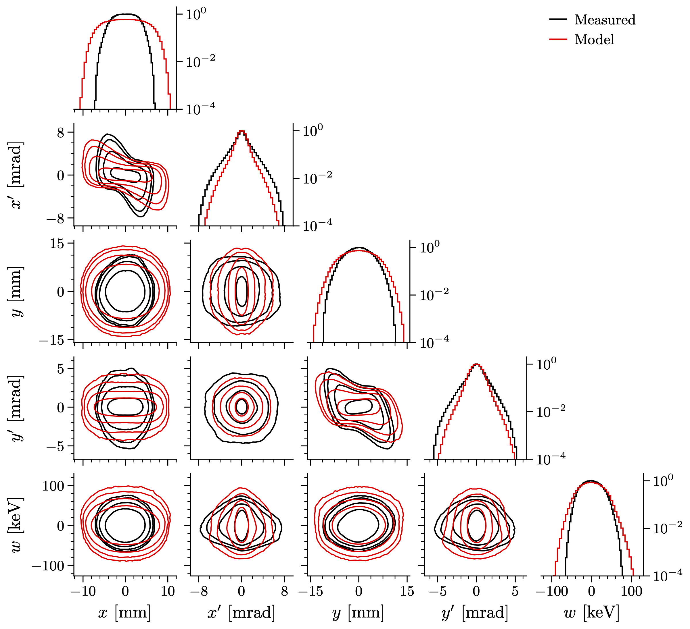
A previous paper found reasonable agreement in high-dimensional slices [5]; I set out to perform a more comprehensive comparison. A year before HB, we performed 5D measurements of the initial beam, mapping the density as a function of \(x\), \(p_x\), \(y\), \(p_y\), and \(p_z\) [6]. The missing dimension, \(z\), is strongly correlated with \(p_z\), so most features are visible from the five measured variables. 5D measurements are much faster than 6D measurements because we can image two dimensions at once on a screen (and because there is one less dimension to measure). Because of the boosted resolution and dynamic range, we can visualize sharper features in low-density regions of phase space.
Here are the 1D and 2D projections of the measured and predicted (PARMTEQ) distributions. Note that I use \(x' = p_x / p_z\) and \(y' = p_y / p_z\) for the transverse momentum. I also use \(w\) instead of \(p_z\), where \(w = E - E_0\) is the deviation from the design energy.
These contours are on a logarithmic scale, showing three orders of magnitude in density. It’s not a total disaster, but it’s kinda bad. Particularly troublesome is the \(x\)-\(p_x\) distribution, which is much wider than measured. However, look what happens after a linear transformation:
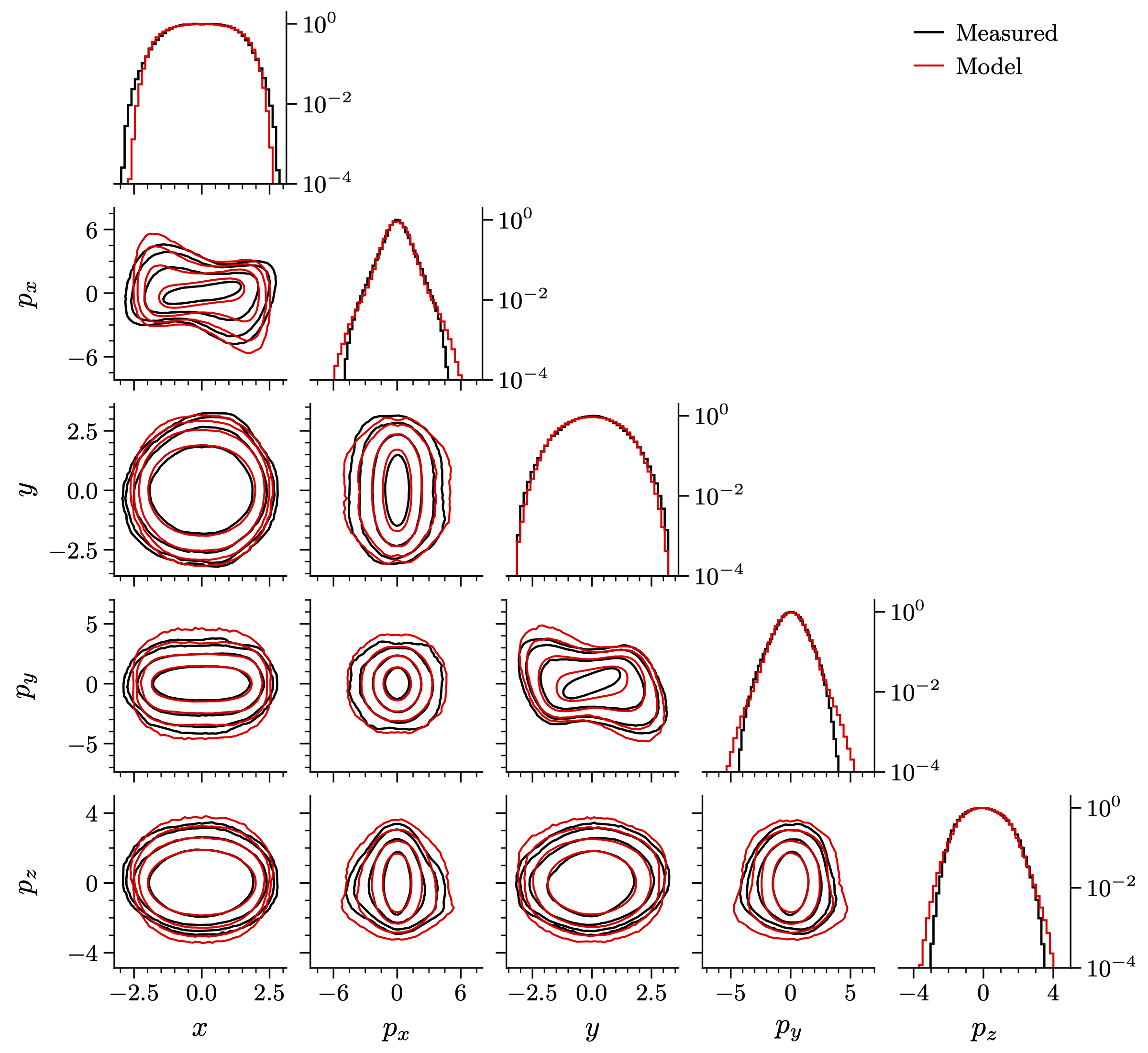
Much better! All I did was normalize both distributions to identity covariance so that
\[\begin{equation} \Sigma = \begin{bmatrix} \langle xx \rangle & \langle xp_x \rangle & \langle xy \rangle & \langle xp_y \rangle & \langle x p_z \rangle \\ \langle xp_x \rangle & \langle p_xp_x \rangle & \langle yp_x \rangle & \langle p_xp_y \rangle & \langle p_xp_z \rangle \\ \langle xy \rangle & \langle yp_x \rangle & \langle yy \rangle & \langle yp_y \rangle & \langle y p_z \rangle \\ \langle xp_y \rangle & \langle p_xp_y \rangle & \langle yp_y \rangle & \langle p_yp_y \rangle & \langle p_yp_z \rangle \\ \langle xp_z \rangle & \langle p_xp_z \rangle & \langle yp_z \rangle & \langle p_yp_z \rangle & \langle p_zp_z \rangle \end{bmatrix} = \begin{bmatrix} 1 & 0 & 0 & 0 & 0 \\ 0 & 1 & 0 & 0 & 0 \\ 0 & 0 & 1 & 0 & 0 \\ 0 & 0 & 0 & 1 & 0 \\ 0 & 0 & 0 & 0 & 1 \end{bmatrix} \end{equation}\]
From now on, I’ll let \(x\), \(p_x\), \(y\), \(p_y\), and \(p_z\) refer to these “normalized” coordinates. Figure 5 shows that the distributions are similar, up to a linear transformation. PARMTEQ has gotten the nonlinear stuff right, even though it predicts a much larger transmission than measured in the real RFQ. This suggests that losses occur very early in the bunch formation process and have little impact on the higher-order distribution moments.
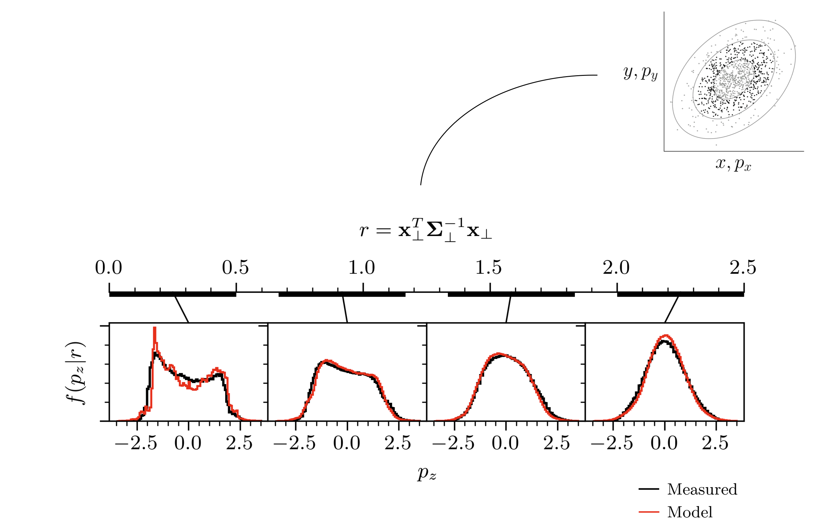
Figure 5 does not prove that the distributions are identical in the full five-dimensional space. There are two higher-dimensional correlations we’ve identified in our 5D measurement. First, we know the energy distribution (\(p_z\)) depends on the transverse coordinates. The energy distribution is bimodal near the transverse core but unimodal outside the core. You can’t see this in the 1D and 2D projections. One way to visualize the relationship is to use “elliptical slices”. Figure 6 shows the \(p_z\) distribution of particles within a radial band in \(x\)-\(p_x\)-\(y\)-\(p_y\) space. The model bunch has the correct relationship between energy and transverse radius.
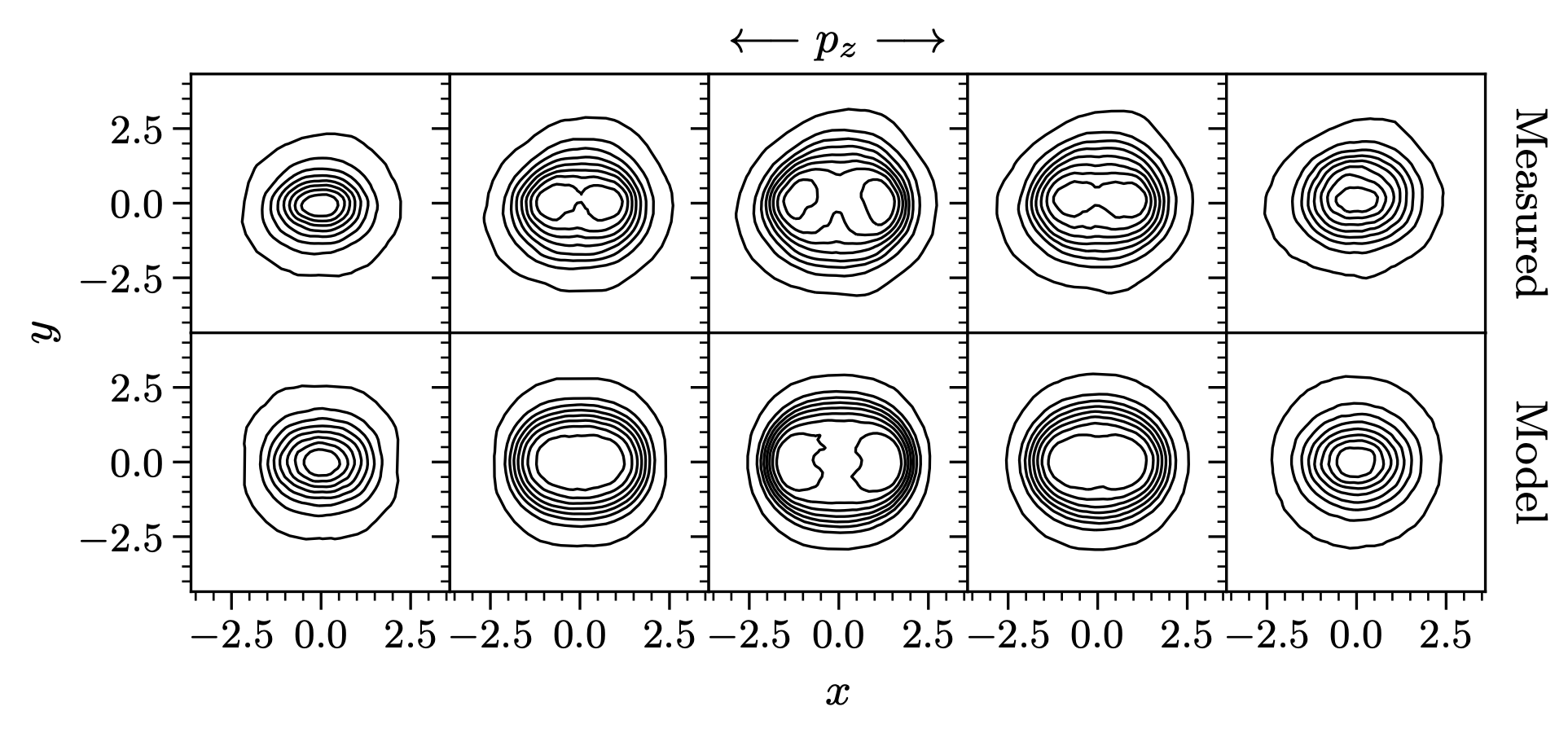
The above feature develops somewhere in the RFQ. We’ve also measured hollowing in the 3D space \(x\)-\(y\)-\(z\). This feature develops after the RFQ. As the beam transitions from strong to weak focusing at the RFQ exit, space charge launches a density wave that flattens the initially peaked distribution to a more uniform and, eventually, hollow distribution. The beam freely expands in the longitudinal plane, creating a strong linear correlation such that (\(z \approx p_z\)). Again, we see similar features in the model bunch in Figure 7. We conclude that the RFQ simulation reproduces nearly all measured features in both low-dimensional and high-dimensional phase space, up to a linear transformation.
This result is interesting and not too obvious; I’d like to include it in a future publication alongside a more detailed study of the beam dynamics in the RFQ. The result is also useful because linear correlations are easy to measure. We can just map the PARMTEQ bunch to the measured linear correlations, and, voila, we have a fully correlated 6D distribution that should be very similar to the real distributioin.
How important are 6D correlations in the SNS linac?
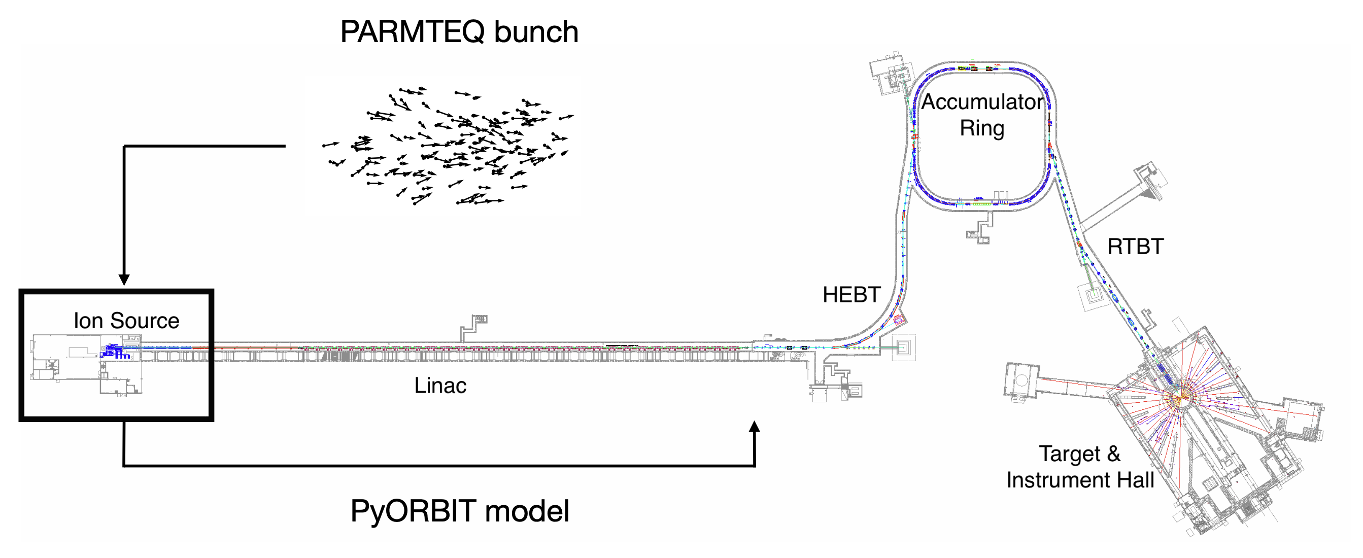
We can also use the model bunch to examine what could happen in the SNS linac. Predicting beam loss in the SNS is our ultimate goal. This is much more difficult than our task in the BTF: the SNS is around 500 meters long compared to 10 meters in the BTF; the SNS accelerates the beam using hundreds of RF cavities, while the BTF has no acceleration; we are much less certain about the accelerator parameters; etc. Figure 8 gives a sense of scale. Still, there is nothing stopping us from assuming, for the sake of argument, that our linac model is correct. We can hypothesize that our physics model is a reasonable approximation of the real world. For example, most people believe the particle-in-cell (PIC) method captures the effect of space charge. We can also imagine a world in which the linac parameters — quadrupole strengths, rf cavity phases, etc. — are equal to the simulation parameters. Finally, in this hypothetical world, we can assume the initial distribution is a linear transformation of the “model” bunch generated by PARMTEQ.
We can now ask how changes to the initial bunch propagate down in the linac. We’re particularly interested in cross-plane correlations. What if we only knew the projected density onto each 2D phase space: \(f(x, p_x)\), \(f(y, p_y)\), and \(f(z, p_z)\)? Without additional information, the only logical 6D distribution compatible with these projections is the product of the 2D distributions (the distribution that maximizes entropy):
\[ \begin{equation} f(x, p_x, y, p_y, z, p_z) = f(x, p_x) f(y, p_y) f(z, p_z). \end{equation} \tag{1}\]
We’ll refer to the bunch in Equation 1 as decorrelated. All cross-plane correlations, including higher-order correlations, vanish in the decorrelated bunch. To decorrelated the bunch, we simply shuffle the particle indices:
\[ \begin{equation} \begin{aligned} \{ x_i, {p_x}_i \} &\rightarrow \{ x_i, {p_x}_i \}, \\ \{ y_i, {p_y}_i \} &\rightarrow \{ y_j, {p_y}_j \}, \\ \{ z_i, {p_z}_i \} &\rightarrow \{ z_k, {p_z}_k \}, \end{aligned} \end{equation} \tag{2}\]
where \(i\), \(j\), and \(k\) are random permutations of the indices.
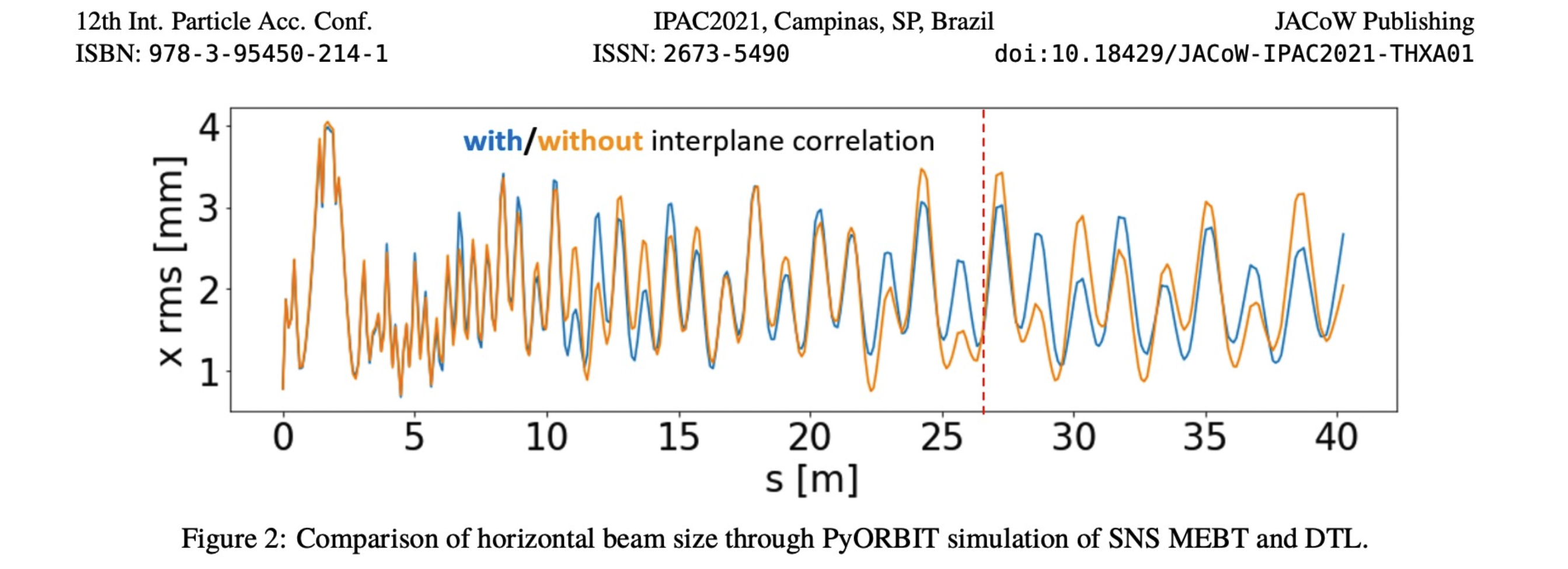
We tracked these two bunches (correlated and decorrelated) through the first section of the linac in our PyORBIT model and compared the trajectories. This isn’t new: my colleague did this in 2021, finding that the two beams diverged in their rms sizes (Figure 9).
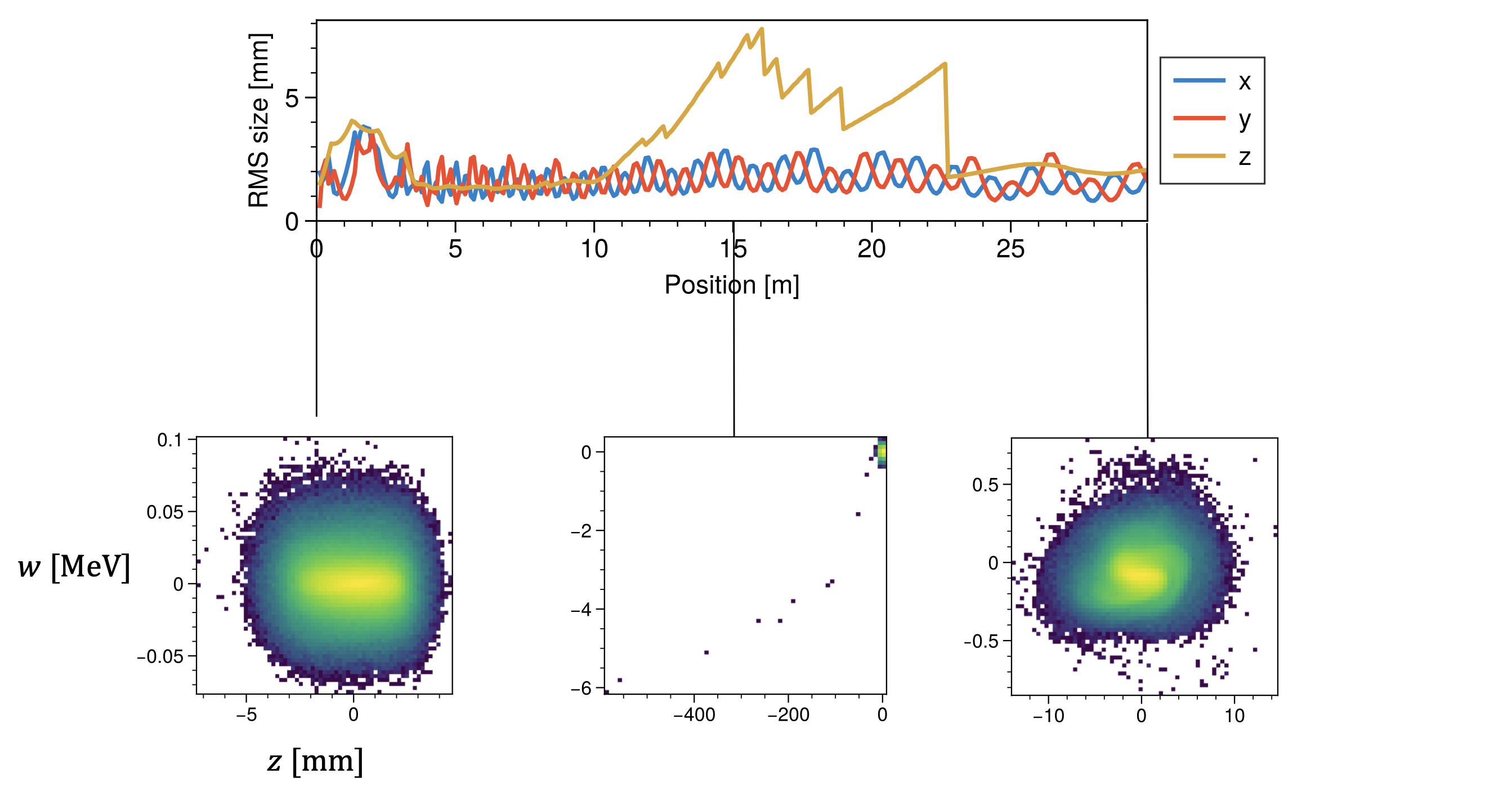
I planned to continue these studies and find out exactly how the 6D phase space correlations influenced the beam dynamics, especially halo formation. When I reproduced Figure 9, though, I noticed something strange. The rms bunch length (\(z\)) spiked halfway through the simulation.
The phase space distributions at these locations showed that some particles were falling way behind the bunch. Eventually, transverse apertures removed these particles from the simulation. It doesn’t make sense to keep these particles in the bunch, so I added energy and phase apertures throughout the lattice to remove particles as soon as they deviated from the synchronous coordinates. Longitudinal apertures ensured a well-behaved rms bunch length, but I no longer saw any differences in the transverse bunch sizes.
What’s going on? It turns out that the lost particles were affecting the space charge calculation. To compute the beam’s electric field, we solve the Poisson equation on a grid:
\[\begin{equation} \nabla \cdot \nabla \phi(x, y, z) = \frac{ \rho(x, y, z) } {\epsilon_0}, \end{equation}\]
where \(\phi\) is the electric potential and \(\rho\) is the charge density. In PyORBIT, the grid expands to include all particles. In Figure 10, the grid would expand in the middle plot to include the \(z\) coordinates behind the bunch. This would leave almost all particles in one \(z\) bin, giving an inaccurate charge density and space charge forces.
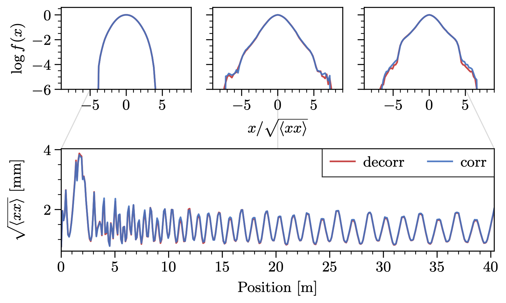
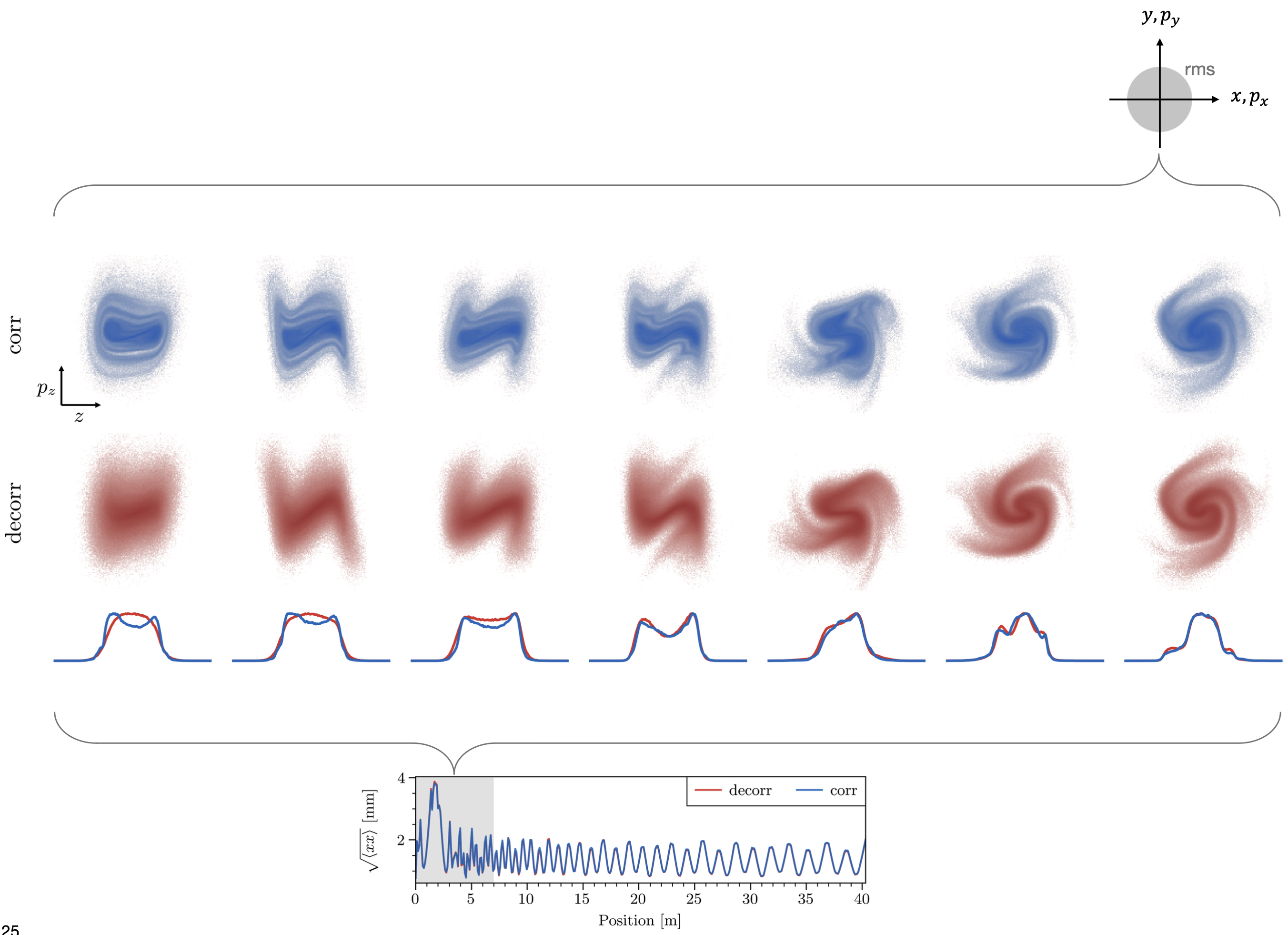
So that’s settled. But it also raises the question: do cross-plane correlations matter at all? Figure 11 shows that the one-dimensional beam density is independent of the initial cross-plane correlations, even at the level of beam halo. Thus the answer is no: according to our model, cross-plane correlations do not affect the beam dynamics in the SNS. The more detailed view in Figure 12 shows that the differences between the distributions disappear quickly, within a few meters. You can see the hollow initial \(z\) distribution in the 1D lineout compared to the peaked \(z\) distribution; this represents a correlation because the distribution is only hollow near \(x = y = p_x = p_y = 0\). The lineouts merge soon after acceleration begins. The distributions are both highly correlated by the end of the figure.
Conclusion
I think these findings are significant. It appears that measuring three orthogonal 2D projections of the 6D distribution can lead to the same predictions as direct 6D measurements. If this is true, we’ll need to direct our attention to the accelerator and physics models in our simulations. Of course, all of this needs experimental validation. Measurements at the BTF will serve as important benchmarks.
Here is the conference paper and slides. Here are the full conference proceedings.
