Coupled parametric oscillators

Author

Austin Hoover

Published

January 25, 2021

A previous post studied the parametric oscillator — an oscillator whose physical properties are time-dependent. The solution was used to describe the transverse oscillations of a charged particle in an accelerator. In this post, the treatment will be extended to coupled parametric oscillators.

Sources of coupling

We’ll consider the following equation of motion:

\[ \begin{aligned} x'' + k_{11}(s)x + k_{13}(s)y + k_{14}(s)y' &= 0, \\ y'' + k_{33}(s)y + k_{31}(s)x + k_{32}(s)x' &= 0, \end{aligned} \tag{1}\]

where the prime denotes differentiation with respect to \(s\), the time-like coordinate. We’ll assume a periodic lattice: \(k_{ij}(s + L) = k_{ij}(s)\) for some distance \(L\). The terms \(k_{13}\), \(k_{31}\), \(k_{14}\), and \(k_{32}\) generate linear coupling between the planes.

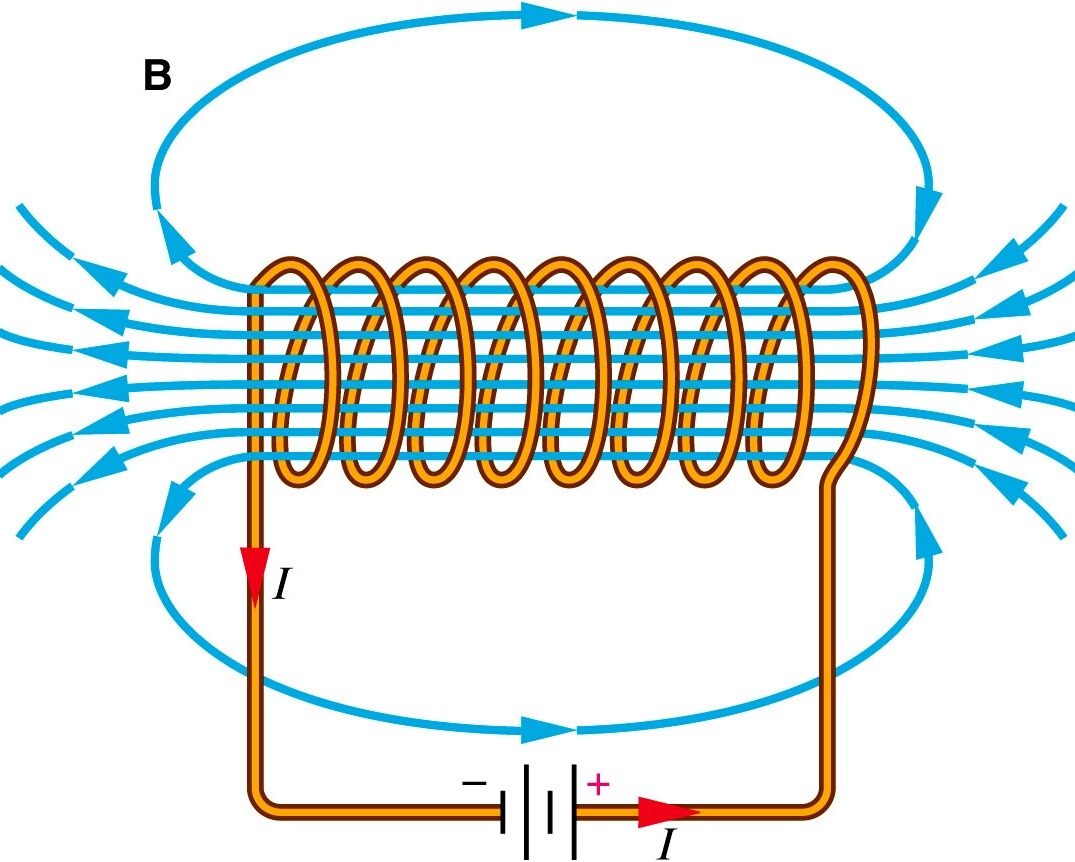
The first potential source of coupling is the longitudinal magnetic field within a solenoid, as shown in Figure 1.


Figure 1: Solenoid magnetic field generated by current loop. (Source: brilliant.org)


For a long solennoid, the field within the coils points in the longitudinal direction and is approximately constant (\(\mathbf{B}_{sol} = B_0\hat{s}\)). From the Lorentz force equation, we find:

\[ m\dot{\mathbf{v}} = q \mathbf{v} \times \mathbf{B} = {qB_0} \left({v_y\hat{x} - v_x\hat{y}}\right). \tag{2}\]

The motion in \(x\) depends on the velocity in \(y\), and vice versa. This corresponds to the \(k_{14}\) and \(k_{32}\) terms in Equation 1.

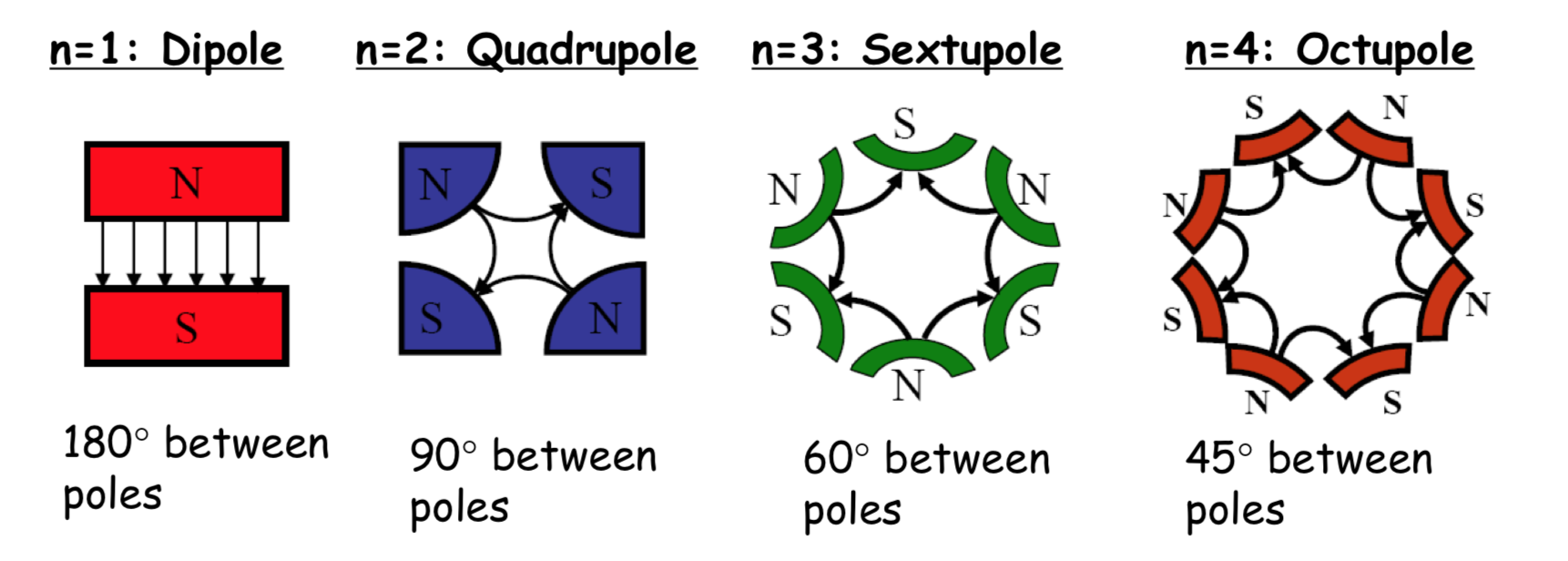
Coupling can also be produced by transverse magnetic fields. Recall the multipole expansion of the transverse magnetic field \(\mathbf{B} = (B_x, B_y)\), shown in Figure 2. There will be nonlinear coupling terms when \(n > 2\), but we are only interested in the linear coupling from the skew quadrupole component. The field couples the force in one plane to the displacement in the other, corresponding to nonzero \(k_{13}\) and \(k_{31}\) terms in Equation 1.

Figure 2: Multipole expansion of the magnetic field up to fourth order.
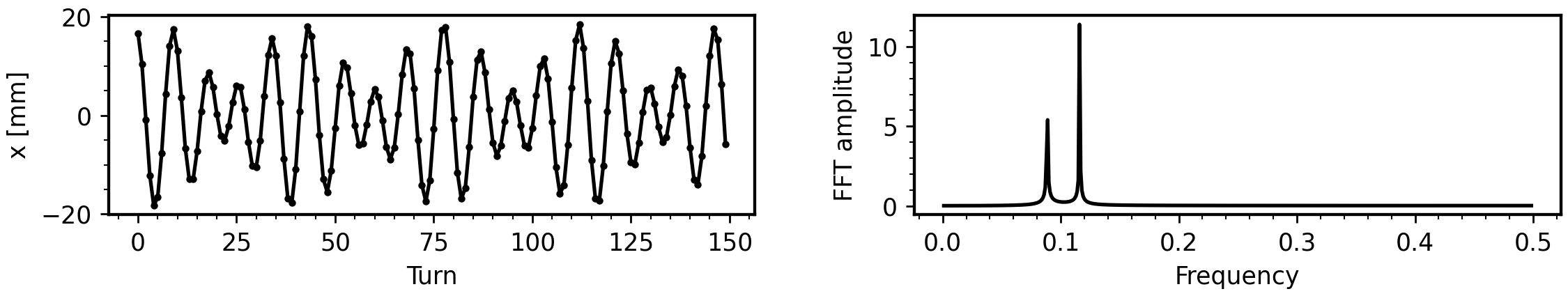
Turn-by-turn data

Let’s review the approach we took in analyzing the one-dimensional parametric oscillator. We wrote the solution in pseudo-harmonic form:

\[ x(s) = \sqrt{2 J \beta(s)} \cos(\mu(s)), \tag{3}\]

with a time-dependent amplitude \(\sqrt{2 J \beta(s)}\) and phase \(\mu(s)\). We then studied the motion of a particle in \(x\)-\(x'\) phase space after each focusing period. We observed that the particle jumps around an ellipse: the area of the ellipse is constant and proportional to \(2 J\); the dimensions of the ellipse are determined by \(\beta\) and \(\alpha = -\beta' / 2\); the size of the jumps around the ellipse are determined by \(\mu\). We then wrote the symplectic \(2 \times 2\) transfer matrix \(\mathbf{M}\), which connects the initial and final phase space coordinates through one period, as

\[ \mathbf{M} = \mathbf{V}\mathbf{P}\mathbf{V}^{-1}. \tag{4}\]

\(\mathbf{V}^{-1}\), which is a function of \(\alpha\) and \(\beta\), is a symplectic transformation that deforms the ellipse into a circle while preserving its area, and \(\mathbf{P}\) is a rotation in phase space by the phase advance \(\mu\).

This is an elegant parameterization of the dynamics. Can we do something similar for coupled motion? To start, let’s track a particle in a lattice with a nonzero skew quadrupole coefficient and plot its phase space coordinates after each turn.

Imports
import matplotlib.animation
import matplotlib.pyplot as plt
import numpy as np
import scipy

plt.rcParams["axes.linewidth"] = 1.25
plt.rcParams["figure.constrained_layout.use"] = True
plt.rcParams["xtick.minor.visible"] = True
plt.rcParams["ytick.minor.visible"] = True
Plotting
class CornerGrid:
    def __init__(self, ndim: int, limits: list[tuple[float, float]] = None, labels: list[str] = None, figwidth: float = None) -> None:
        self.ndim = ndim       

        # Create figure
        if figwidth is None:
            figwidth = 2.0 * (self.ndim - 1)
            
        self.fig, self.axs = plt.subplots(ncols=(ndim - 1), nrows=(ndim - 1), figsize=(figwidth, figwidth), sharex="col", sharey="row")

        # Turn off upper-diagonal plots.
        for i in range(self.ndim - 1):
            for j in range(self.ndim - 1):
                if i < j:
                    self.axs[i, j].axis("off")

        # Remove top/right spines.
        for ax in self.axs.flat:
            for loc in ["top", "right"]:
                ax.spines[loc].set_visible(False)

        # Set axis limits and labels.
        self.limits = None
        self.labels = None
        self.set_limits(limits)
        self.set_labels(labels)
        
    def set_limits(self, limits: list[tuple[float, float]] = None) -> None:
        if limits is None:
            return
            
        self.limits = limits
        for j in range(self.ndim - 1):
            for ax in self.axs[:, j]:
                ax.set_xlim(self.limits[j])
        for i in range(self.ndim - 1):
            for ax in self.axs[i, :]:
                ax.set_ylim(self.limits[i + 1])

    def set_labels(self, labels: list[str] = None) -> None:
        if labels is None:
            return
            
        self.labels = labels
        for j in range(self.ndim - 1):
            self.axs[-1, j].set_xlabel(self.labels[j])
        for i in range(self.ndim - 1):
            self.axs[i, 0].set_ylabel(self.labels[i + 1])

        self.fig.align_xlabels()
        self.fig.align_ylabels()
            
    def plot_scatter(self, points: np.ndarray, **kws) -> None:
        for i in range(self.ndim - 1):
            for j in range(self.ndim - 1):
                ax = self.axs[i, j]
                if i >= j:
                    ax.scatter(points[:, j], points[:, i + 1], **kws)
        self.set_limits(self.limits)

        
def plot_vector(
    vector: np.ndarray,
    origin: tuple[float] = (0.0, 0.0),
    color: str = "black",
    lw: float = None,
    style: str = "->",
    head_width: float = 0.4,
    head_length: float = 0.8,
    ax=None,
) -> None:
    props = dict()
    props["arrowstyle"] = f"{style},head_width={head_width},head_length={head_length}"
    props["shrinkA"] = props["shrinkB"] = 0
    props["fc"] = props["ec"] = color
    props["lw"] = lw

    vector = np.copy(vector)
    vector = np.add(vector, origin)
    ax.annotate("", xy=(vector[0], vector[1]), xytext=origin, arrowprops=props)


def animate_corner(
    particles: np.ndarray, 
    vectors: list[list[np.ndarray]] = None, 
    limits: list[tuple[float, float]] = None, 
    vector_kws: dict = None, 
    **kws
) -> matplotlib.animation.FuncAnimation:
    
    # Set plot limits.
    if limits is None:
        xmax = np.max(particles, axis=0)
        xmax = xmax * 1.4
        xmax[0] = xmax[2] = max(xmax[0], xmax[2])
        xmax[1] = xmax[3] = max(xmax[1], xmax[3])
        limits = list(zip(-xmax, xmax))

    # Set plot labels.
    labels = ["x", "x'", "y", "y'"]

    # Set default key word arguments.
    if vector_kws is None:
        vector_kws = dict()
    vector_kws.setdefault("head_width", 0.2)
    vector_kws.setdefault("head_length", 0.4)
    
    kws.setdefault("marker", ".")
    kws.setdefault("mec", "None")
    kws.setdefault("lw", 0.0)
    kws.setdefault("color", "black")
    kws.setdefault("ms", 5.0)

    # Create figure
    grid = CornerGrid(ndim=4, figwidth=6.0, limits=limits, labels=labels)

    new_lines = [[], [], []]
    old_lines = [[], [], []]
    for i in range(3):
        for j in range(i + 1):
            ax = grid.axs[i, j]
            
            old_line, = ax.plot([], [], alpha=0.25, **kws)
            old_lines[i].append(old_line)
            
            new_line, = ax.plot([], [], **kws)
            new_lines[i].append(new_line)

    plt.close()

    # Define update rule
    def update(frame):
        for ax in grid.axs.flat:
            for annotation in ax.texts:
                annotation.set_visible(False)

        x = particles[frame]
        for i in range(3):
            for j in range(i + 1):
                ax = grid.axs[i, j]

                axis = (j, i + 1)
                old_lines[i][j].set_data(particles[:frame, axis[0]], particles[:frame, axis[1]])
                new_lines[i][j].set_data((x[axis[0]],), (x[axis[1]],))
                
                if vectors is not None:
                    v1 = vectors[0][frame]
                    v2 = vectors[1][frame]
                    v1_proj = v1[[axis[0], axis[1]]]
                    v2_proj = v2[[axis[0], axis[1]]]
                    plot_vector(
                        v1_proj,
                        origin=(0, 0), 
                        color="blue", 
                        ax=ax, 
                        **vector_kws
                    )
                    plot_vector(
                        v2_proj,
                        origin=v1_proj,
                        color="red",
                        ax=ax,
                        **vector_kws
                    )
                    
        grid.axs[0, 1].annotate(
            "Period {}".format(frame),
            xy=(0.5, 0.5),
            xycoords="axes fraction",
            horizontalalignment="center",
        )

    return matplotlib.animation.FuncAnimation(grid.fig, update, frames=particles.shape[0])
Tracking
def build_poisson_matrix(ndim: int = 4) -> None:
    U = np.zeros((ndim, ndim))
    for i in range(0, ndim, 2):
        U[i : i + 2, i : i + 2] = [[0.0, 1.0], [-1.0, 0.0]]
    return U


def normalize_eigvec(v: np.ndarray) -> np.ndarray:
    ndim = v.shape[0]
    U = build_poisson_matrix(ndim)
    norm = np.abs(np.imag(np.linalg.multi_dot([np.conj(v), U, v])))
    if norm > 0:
        return v * np.sqrt(2.0 / norm)
    return v

    
def build_norm_matrix_from_eigvecs(v1: np.ndarray, v2: np.ndarray) -> np.ndarray:
    v1 = normalize_eigvec(v1)
    v2 = normalize_eigvec(v2)
    
    V = np.zeros((4, 4))
    V[:, 0] = +v1.real
    V[:, 1] = -v1.imag
    V[:, 2] = +v2.real
    V[:, 3] = -v2.imag
    return np.linalg.inv(V)


def build_norm_matrix_from_tmat(M: np.ndarray) -> np.ndarray:
    eig_res = np.linalg.eig(self.M)
    v1 = normalize_eigvec(eig_res.eigenvectors[:, 0])
    v2 = normalize_eigvec(eig_res.eigenvectors[:, 2])
    return build_norm_matrix_from_eigvecs(v1, v2)
    

def rotate_matrix(M: np.ndarray, angle: float) -> np.ndarray:
    c = np.cos(angle)
    s = np.sin(angle)
    R = np.array([[c, 0, s, 0], [0, c, 0, s], [-s, 0, c, 0], [0, -s, 0, c]])
    return np.linalg.multi_dot([np.linalg.inv(R), M, R])


def build_matrix_drift_2d(length: float) -> np.ndarray:
    return np.array([[1.0, length], [0.0, 1.0]])

    
def build_matrix_drift(length: float) -> np.ndarray:
    matrix = np.zeros((4, 4))
    matrix[0:2, 0:2] = build_matrix_drift_2d(length)
    matrix[2:4, 2:4] = build_matrix_drift_2d(length)
    return matrix


def build_matrix_quad_2d(length: float, k: float) -> np.ndarray:
    sign = np.sign(k)
    k = np.sqrt(np.abs(k))

    matrix = np.zeros((2, 2))
    if sign >= 0:        
        matrix[0, 0] = +np.cos(k * length)
        matrix[0, 1] = +np.sin(k * length) / k
        matrix[1, 0] = -np.sin(k * length) * k
        matrix[1, 1] = +np.cos(k * length)
    else:
        matrix[0, 0] = +np.cosh(k * length)
        matrix[0, 1] = +np.sinh(k * length) / k
        matrix[1, 0] = +np.sinh(k * length) * k
        matrix[1, 1] = +np.cosh(k * length)
    return matrix
    

def build_matrix_quad(length: float, k: float, tilt: float = 0.0) -> np.ndarray:
    matrix = np.zeros((4, 4))
    matrix[0:2, 0:2] = build_matrix_quad_2d(length, +k)
    matrix[2:4, 2:4] = build_matrix_quad_2d(length, -k)
    if tilt:
        matrix = rotate_matrix(matrix, tilt)
    return matrix

    
class Lattice:
    def __init__(self):
        self.matrices = []
        self.M = None
        self.V = None
        self.V_inv = None
        self.eigvec_1 = None
        self.eigvec_2 = None
        self.eigval_1 = None
        self.eigval_2 = None
        self.params = dict()

    def length(self) -> int:
        return len(self.matrices)

    def add(self, matrix: np.ndarray) -> None:
        self.matrices.append(matrix)
        self.build()

    def build(self) -> None:
        length = self.length()
        if length == 0:
            return
        elif length == 1:
            self.M = self.matrices[0]
        else:
            self.M = np.linalg.multi_dot(list(reversed(self.matrices)))

    def analyze(self) -> None:
        result = np.linalg.eig(self.M)
        self.eigval_1 = result.eigenvalues[0]
        self.eigval_2 = result.eigenvalues[2]
        self.eigvec_1 = normalize_eigvec(result.eigenvectors[:, 0])
        self.eigvec_2 = normalize_eigvec(result.eigenvectors[:, 2])
        self.V_inv = build_norm_matrix_from_eigvecs(self.eigvec_1, self.eigvec_2)
        self.V = np.linalg.inv(self.V_inv)
        
    def normal_form(self) -> None:
        return np.linalg.multi_dot([self.V_inv, self.M, self.V])

    def track(self, x: np.ndarray, turns: int = 1, normalize: bool = False):
        M = np.copy(self.M)
        if normalize:
            x = np.matmul(self.V_inv, x)
            M = self.normal_form()
            
        X = np.zeros((turns + 1, x.shape[0]))
        X[0, :] = np.copy(x)
        for i in range(1, turns):
            X[i, :] = np.matmul(M, X[i - 1, :])
        return X


def build_fodo_lattice(length: float, k: float, quad_tilt: float = 0) -> Lattice:
    length = 0.125 * length
    
    lattice = Lattice()
    lattice.add(build_matrix_drift(length))
    lattice.add(build_matrix_quad(length, +k, tilt=+quad_tilt))
    lattice.add(build_matrix_quad(length, +k, tilt=+quad_tilt))
    lattice.add(build_matrix_drift(length))
    lattice.add(build_matrix_drift(length))
    lattice.add(build_matrix_quad(length, -k, tilt=-quad_tilt))
    lattice.add(build_matrix_quad(length, -k, tilt=-quad_tilt))
    lattice.add(build_matrix_drift(length))
    return lattice


# Generate a FODO lattice. The quadrupoles are tilted to generate x-y coupling.
lattice = build_fodo_lattice(length=5.0, k=0.25, quad_tilt=np.radians(-1.0))
lattice.analyze()

# Set initial particle coordinates. Three particles: v1, v2, v1 + v2.
action_1 = 0.5 * 40.0  # mode 1 amplitude
action_2 = 0.5 * 10.0  # mode 2 amplitude
phase_1 = np.pi * 0.00  # mode 1 phase
phase_2 = np.pi * 0.25  # mode 2 phase
x_1 = np.real(np.sqrt(2.0 * action_1) * lattice.eigvec_1 * np.exp(1.0j * phase_1))
x_2 = np.real(np.sqrt(2.0 * action_2) * lattice.eigvec_2 * np.exp(1.0j * phase_2))
x = x_1 + x_2

# Track particles 1000 turns and store turn-by-turn coordinates.
turns = 1000
particles_1 = lattice.track(x_1, turns)
particles_2 = lattice.track(x_2, turns)
particles = lattice.track(x, turns)

# Animate first 45 turns in corner plot.
turns_plot = 45

xmax = 1.4 * np.max(particles, axis=0)
xmax[0] = xmax[2] = max(xmax[0], xmax[2])
xmax[1] = xmax[3] = max(xmax[1], xmax[3])
limits = list(zip(-xmax, xmax))

animation = animate_corner(particles[:turns_plot, :], limits=limits);
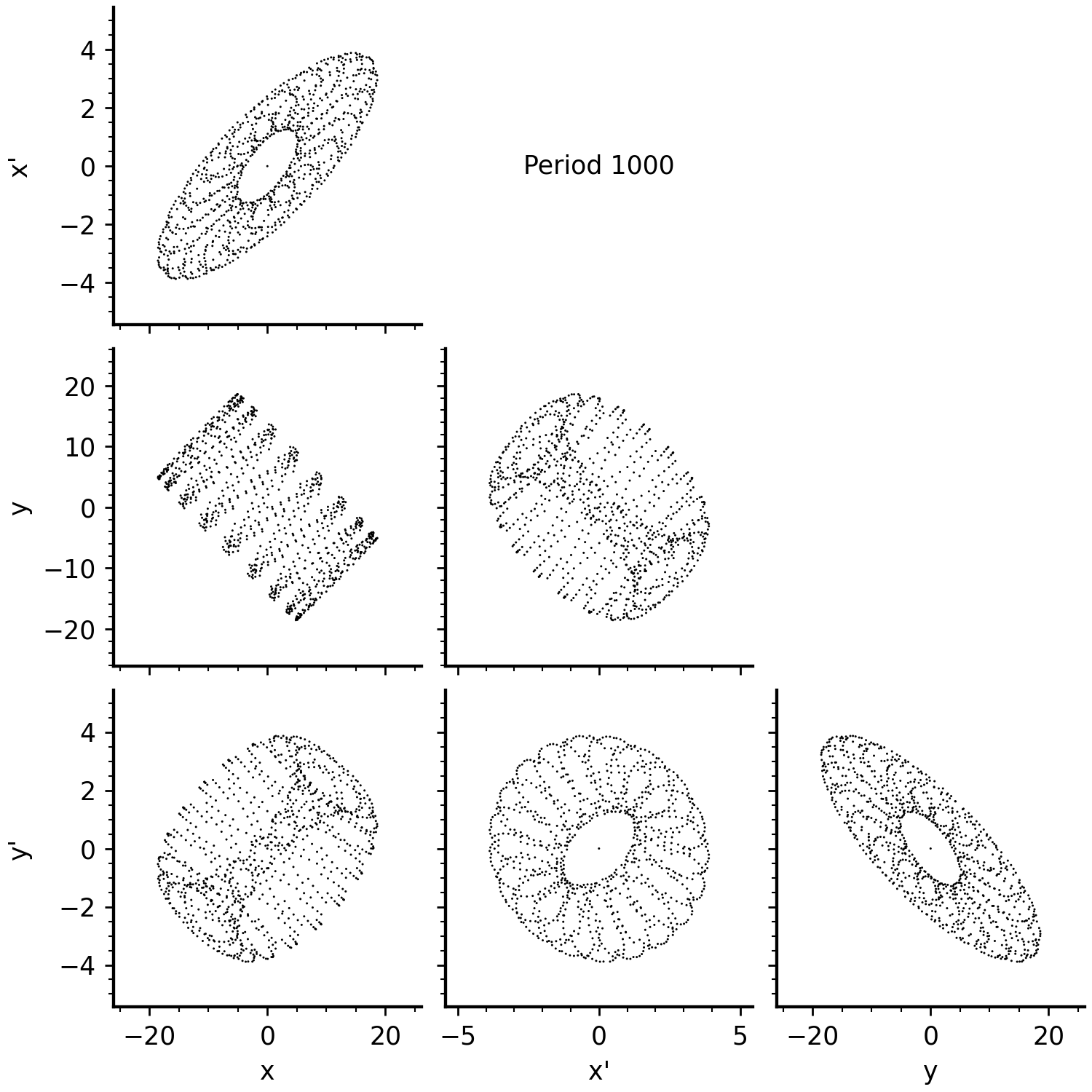
Figure 3: Period-by-period four-dimensional phase space coordinates of a coupled parametric oscillator.

Figure 3 shows the 2D projections of the turn-by-turn coordinates. Instead of ellipses, the particle traces donut-like shapes in the \(x\)-\(x'\) and \(y\)-\(y'\) planes. Figure 4 shows the result after 1000 turns.

Code
grid = CornerGrid(ndim=4, figwidth=6.0, limits=limits, labels=["x", "x'", "y", "y'"])
grid.plot_scatter(particles, s=0.75, c="black", ec="none")
grid.axs[0, 1].annotate(
    "Period 1000",
    xy=(0.5, 0.5),
    xycoords="axes fraction",
    horizontalalignment="center",
    verticalalignment="center",
)
plt.close();
Figure 4: Phase space coordates after 1000 periods.

There’s clearly more than one frequency present. Here’s the FFT of the horizontal coordinate \(x\):

Code
n = particles.shape[0]
m = n // 2
f = (1.0 / n) * np.arange(m)
xf = (1.0 / m) * abs(scipy.fft.fft(particles[:, 0])[:m])

fig, axs = plt.subplots(ncols=2, figsize=(9.0, 1.7), sharey=False, gridspec_kw=dict(wspace=0.1))
axs[0].plot(particles[:150, 0], color="black", marker=".", ms=4)
axs[0].set_xlabel("Turn")
axs[0].set_ylabel("x [mm]")
axs[1].plot(f[1:], xf[1:], color="black")
axs[1].set_xlabel("Frequency")
axs[1].set_ylabel("FFT amplitude")
plt.close()

This is a signature of a linearly coupled oscillator. The motion in coupled systems can be understood as the superposition of normal modes, each of which corresponds to a single frequency. For example, consider two masses connected with a spring. There are two possible ways for the masses to oscillate at the same frequency. The first is a breathing mode in which they move in opposite directions, and the second is a sloshing mode in which they move in the same direction. The actual motion is the sum of these two modes. We will try to do something similar for a coupled parameteric oscillator.

Eigenvector analysis

The phase space coordinate vector \(\mathbf{x} = (x, x', y, y')^T\) evolves according to

\[ \mathbf{x} \rightarrow \mathbf{Mx}, \tag{5}\]

where \(\rightarrow\) represents tracking through one period. It can be shown that \(\mathbf{M}\) is symplectic due to the Hamiltonian mechanics of the system. Consider the eigenvectors of \(\mathbf{M}\):

\[ \mathbf{Mv}_k = \lambda_k \mathbf{v}_k = e^{-i\mu_k} \mathbf{v}_k. \tag{6}\]

The symplectic condition leads to a degeneracy of the eigenvalues and eigenvectors: they can be grouped into pairs related by complex conjugation. This means we can label the eigenvalues as \(\{\lambda_k, \lambda_k^* \}\) and eigenvectors as \(\{\mathbf{v}_k, \mathbf{v}_k^* \}\) for \(k = 1, 2\). We can write any coordinate vector as a linear combination of the real and imaginary components of \(\mathbf{v}_1\) and \(\mathbf{v}_2\):

\[ \mathbf{x} = \text{Re} \left\{ \sqrt{2 J_1}\mathbf{v}_1e^{-i\psi_1} + \sqrt{2 J_2}\mathbf{v}_2e^{-i\psi_2} \right\}, \tag{7}\]

where \(\text{Re}\{\dots\}\) selects the non-imaginary component. We have introduced two invariant amplitudes (\(J_1\) and \(J_2\)) as well as two initial phases (\(\psi_1\) and \(\psi_2\)). The transfer matrix \(\mathbf{M}\)% simply tacks on a phase to each eigenvector.

\[ \mathbf{Mx} = \text{Re} \left\{ \sqrt{2 J_1}\mathbf{v}_1e^{-i\left(\psi_1 + \mu_1\right)} + \sqrt{2 J_2}\mathbf{v}_2e^{-i(\psi_2 + \mu_2)} \right\}. \tag{8}\]

Let’s replay the corner plot animation, but this time draw a blue arrow for \(\mathbf{v}_1\) and a red arrow for \(\mathbf{v}_2\). I’ve chosen initial amplitudes \(J_1 = 4 J_2\) and phases \(\psi_2 - \psi_1 = \pi/2\).

Code
animation = animate_corner(particles[:turns_plot, :], limits=limits, vectors=[particles_1, particles_2]);
Figure 5: Turn-by-turn coordinates with eigenvector projections as blue/red arrows.

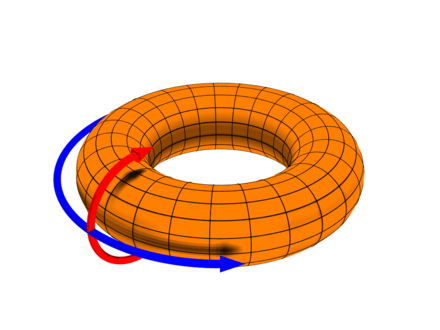
Much simpler. Each eigenvector \(\mathbf{v}_k\) simply rotates in the complex plane at its frequency \(\mu_k\). It also explains why the amplitudes in the \(x\)-\(x'\) and \(y\)-\(y'\) planes trade back and forth: the eigenvector projections rotate at different frequencies, sometimes aligning and sometimes anti-aligning. The amplitudes \(J_{1, 2}\) are generalizations of the Courant-Snyder (CS) invariants \(J_{x, y}\) derived for uncoupled focusing. In the four-dimensional phase space, the amplitudes define an inner and outer “radius” of an invariant four-dimensional torus. The phases simply define a point on the torus.

Figure 6: Representation of the invariant torus in four-dimensional phase space.

Eigenvector parameterization

In the previous analysis of uncoupled systems, we parameterized the normalization matrix \(\mathbf{V}\) using the so-called Courant-Synder (CS) parameters \(\alpha\) and \(\beta\). We can also come up with four-dimensional parameterizations, but there is no universally agreed-upon method to do this. The following is the method described by Lebedev and Bocacz in  [1].

First, since the eigenvectors are related to the transfer matrix, they must also be related to the normalization matrix \(\mathbf{V}\). Indeed, \(\mathbf{V}\) is constructed from \(\mathbf{v}_1\) and \(\mathbf{v_2}\) as follows:

\[ \mathbf{V} = \left[ +\Re\{\mathbf{v}_1\} -\Im\{\mathbf{v}_1\} +\Re\{\mathbf{v}_2\} -\Im\{\mathbf{v}_2\} \right], \]

where \(\Re\) and \(\Im\) select the real and imaginary components, respectively. So parameterizing the normalization matrix is equivalent to parameterizing the eigenvectors.

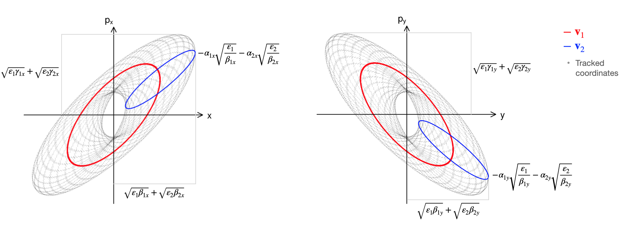
To motivate the parameterization, notice that each eigenvector traces an ellipse in both the horizontal (\(x\)-\(x'\)) and vertical (\(y\)-\(y'\)) phase planes. Let’s assign an \(\alpha\) and \(\beta\) parameter to each of the four ellipses. For the ellipse traced by \(\mathbf{v}_1\) in the \(x\)-\(x'\) plane, we have \(\beta_{1x}\) and \(\alpha_{1x}\), and then for the second eigenvector we have \(\beta_{2x}\) and \(\alpha_{2x}\). For the ellipse traced by \(\mathbf{v}_1\) in the \(y\)-\(y'\) plane, we have \(\beta_{1y}\) and \(\alpha_{1y}\), and then for the second eigenvector we have \(\beta_{2y}\) and \(\alpha_{2y}\). See Figure 7.

Figure 7: Four-dimensional Twiss parameters. Each eigenvector traces an ellipse in each two-dimensional plane (\(x\)-\(x'\), \(y\)-\(y'\)); each ellipse is assigned an \(\alpha\) and \(\beta\) parameter.

We can then write the eigenvectors in terms of the alpha and beta functions, plus a few more parameters:

\[ \mathbf{v}_1 = \begin{bmatrix} \sqrt{\beta_{1x}} \\ -\frac{\alpha_{1x} + i(1-u)}{\sqrt{\beta_{1x}}} \\ \sqrt{\beta_{1y}}e^{i\nu_1} \\ -\frac{\alpha_{1y} + iu}{\sqrt{\beta_{1y}}} e^{i\nu_1} \end{bmatrix}, \quad \mathbf{v}_2 = \begin{bmatrix} \sqrt{\beta_{2x}}e^{i\nu_2} \\ -\frac{\alpha_{2x} + iu}{\sqrt{\beta_{2x}}}e^{i\nu_2} \\ \sqrt{\beta_{2y}} \\ -\frac{\alpha_{2y} + i(1-u)}{\sqrt{\beta_{2y}}} \end{bmatrix} \tag{9}\]

The additional parameters are not independent. The first additional parameter is \(u\), which determines the areas of the ellipses in one plane relative to the other. The second and third additional parameters are \(\nu_1\) and \(\nu_2\), which are phase differences between the \(x\) and \(y\) components of the eigenvectors (in the animation they are either \(0\) or \(\pi\)). I won’t discuss these here.

The last thing to note is that the parameters reduce to their 1D counterparts when there is no coupling in the lattice: \(\beta_{1x}, \beta_{2y} \rightarrow \beta_{x}, \beta_{y}\) and \(\beta_{2x}, \beta_{1y} \rightarrow 0\) (similar for \(\alpha\)). The invariants and phase advances would also revert back to their original definitions: \(J_{1,2} \rightarrow J_{x,y}\) and \(\mu_{1,2} \rightarrow \mu_{x,y}\).

Floquet transformation

The eigenvectors/normalization matrix can be used to construct a transformation that removes both the \(s\)-dependence of the focusing strength and coupling between planes, transforming the coupled parametric oscillator into an uncoupled harmonic oscillator.

\[\mathbf{V^{-1} M V} = \mathbf{P} = \begin{bmatrix} \cos{\mu_1} & \sin{\mu_1} & 0 & 0 \\ -\sin{\mu_1} & \cos{\mu_1} & 0 & 0 \\ 0 & 0 & \cos{\mu_2} & \sin{\mu_2} \\ 0 & 0 & -\sin{\mu_2} & \cos{\mu_2} \end{bmatrix} \tag{10}\]

We can do this simply by rewriting Equation 7 as \(\mathbf{x} = \mathbf{V}\mathbf{u}\) with

\[ \mathbf{u} = \begin{bmatrix} +\sqrt{2J_1}\cos{\psi_1} \\ -\sqrt{2J_1}\sin{\psi_1} \\ +\sqrt{2J_2}\cos{\psi_2} \\ -\sqrt{2J_2}\sin{\psi_2} \end{bmatrix}. \tag{11}\]

Let’s observe the motion in the normalized coordiantes \(\mathbf{u} = [u_1, u_1', u_2, u_2']\).

Code
x = x_1 + x_2

particles = lattice.track(x, turns, normalize=True)
particles_1 = lattice.track(x_1, turns, normalize=True)
particles_2 = lattice.track(x_2, turns, normalize=True)
particles_1[:, 2:4] *= 0
particles_2[:, 0:2] *= 0

animation = animate_corner(particles[:turns_plot, :], vectors=[particles_1, particles_2]);
Figure 8: Period-by-period motion in normalized/Floquet coordinates

The motion is uncoupled after this transformation; i.e., particles move in a circle of area \(2J_1\) in the \(u_1\)-\(u_1'\) plane at frequency \(\mu_1\), and in a circle of area \(2J_2\) in the \(u_1\)-\(u_1'\) plane at frequency \(\mu_2\).

Conclusion

This post has described the eigenvector analysis of linear parametric oscillators. Note that the Lebedev-Bogacz parameterization  [1] isn’t the only choice; it’s just what I’ve used in my own research. There’s also a more recent formulation that doesn’t use eigenvectors at all  [2]. But I think I would need to learn some math (group theory) to understand that approach.

No matching items

References

[1]
V. A. Lebedev and S. Bogacz, Betatron Motion with Coupling of Horizontal and Vertical Degrees of Freedom, Journal of Instrumentation 5, P10010 (2010).
[2]